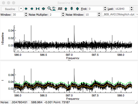
Procedures Automatic Fitting <Prev Next>

Automatic Fitting of an N2O IR Spectrum

This walk through shows how to use the automatic assignment process on the N2O sample file provided in the Walk-through of Simulating and Fitting a Simple Spectrum (which this assumes you are familar with).

  1. Load the overlay N2Onu2.ovr.
  2. Right click on the overlay and select "Baseline...".
  3. Use the zoom buttons to zoom in on a small sample of the spectrum to show the (small) baseline ripple. (The zoom buttons in this window work in the same way as the in the main window.)
  4. Press the "Baseline" button to calculate a baseline. The orange line shows the calculated baseline, and the green line indicates the upper limit of the points used in calculating the baseline. The upper pane shows the spectrum after subtracting the baseline. The expand vertical button () can be helpful in expanding the baseline. Experiment with the "Window", "Noise Multiplier", and possibly the "Noise Window" settings and with "Dense" selected from the drop down menu. (Click on the down arrow next to the "Baseline" button to see this.) You need to click on the "Baseline" button after changing the settings to update the display. The baseline algorithm works by attempting to identify points on the baseline (within the noise multiplier) and taking a moving average over the window. A "Window" of 30, "Noise Multiplier" of 2 and selecting "Dense" gives good results for this spectrum:
  5. If you want to save the spectrum with the baseline subtracted, select "Apply to New" from the drop down menu to generate an overlay with a flat baseline.
  6. To make a line list, adjust the "Noise Multiplier" so that the green line is above almost all of the noise. It is not necessarily the same as used for the baseline calculation - in this case a "Noise Multiplier" of 3 is promising. Selecting "Live update" from the drop down menu will show the lines found in the upper window in blue automatically as the parameters are changed, though note this can be slow if the selected region is large.
  7. When you are happy with the result, generate the linelist by selecting "Make Line list" from the drop down menu. The resulting line list will be added to the overlays, and show in the main window.
  8. In the current example, the above settings give bad results for a few regions where the noise is larger, so re-run the peak finder over smaller regions as follows:
    1. Select the region to update by either:
      1. Select a region in the baseline window
      2. Make this the active region for peak finding by selecting "Select Visible" from the drop down menu.
      or:
      1. Select a region in the main window, and zoom the main window to that region
      2. Make this the active region for peak finding by selecting "Load Visible" from the drop down menu in the baseline window.
    2. Adjust the noise window as required.
    3. To replace the peaks in the line list, select "Append Linelist To..." from the drop down menu, making sure the generated line list is selected and "Erase Current Region" is checked when prompted.
    4. Repeat as required - to reset the window, select "Load All" in the drop down menu.
  9. To delete individual lines from the line list in the main window, right click on the line and select "Delete Point"
  10. To delete several adjacent lines, select them (left click and drag) and then right click and select "Delete Points".
  11. To add individual lines by manual measurement, right click and drag over the peak in the baseline window.
  12. The original experimental spectrum is not required at this point - you may want to hide or remove it from the main window by right clicking on it and selecting the appropriate option. You may want to use it later, though, for checking for weak peaks that the automatic peak finder may have missed.
  13. The line list is saved as N2Onu2lin.ovr, using "Save Overlay As...".
To autofit, try fitting to a few P and R branch lines only:
  1. Generate the basic molecule type with File, New, Linear molecule and set Upper State = Pi
  2. Try B"= 0.45, B' = 0.451, Origin = 588.7 for an approximate simulation. These should have "Float" = yes. (The values are not at all critical but the simulation should look qualitatively correct.)
  3. Right click on (say) one P and two R branch lines, and then a few more of each.
  4. In the line list window, select "More, Advanced" to make the autofit options visible. The key setting is the "Accept" window to the maximum error you expect for the "check" transitions. The default (0.1) may be good, but something of the order of the linewidth (here 0.001) might be better.
  5. Select the "fit" lines in the line list window by clicking and dragging with the mouse in the left hand column:
    The first three lines make a good start - there must be at least as many as there are floated parameters. The unselected lines are the "check" transitions.
  6. Bring up the auto fit window with "Overlays, Autofit..."
  7. In this window, the "Window" is the search window for the initial fits, i.e. how far each side of the initial "fit" line positions you want to search. This should reflect how far out you think the lines might be - try 3 cm-1.
  8. We can now try an autofit. The file at this stage (before the autofit) is available as N2Oauto1.pgo.
  9. Press "Search" - after a short while, the window will list, for the best fits found:
    • nOK - the number of "check" transitions within the "Accept" window
    • Residual - the RMS observed - calculated for these "check" transitions.
    • SumI - the sum of observed intensity for these "check" transitions.
    • The values of the constants obtained for each fit.
    • Trial - The number of the trial. (This is typically only useful for debugging purposes.)
    • nDiff - the number of transitions different to the selected fit. This is only displayed if one of the fits is selected.
    Some additional information is shown in the log window.
  10. To try out an individual fit, double click on that row. This will update the line list window with all the assignments made by that fit, and the standard PGOPHER fit process can then be used to refine the fit. Providing the original set of lines are not deleted from the line list window, this process can be used to start other fits at any time. If you don't like the result, the "Reset" button will discard the new assignments and reset the parameters. For the sample saved, most of the fits look more or less OK, but only fit number 4 has the Q branch origin in the right place.
  11. If you want to limit the possible range for parameter values, set the maximum permitted change (+ or -) as the "Std Dev" in the constants window for the parameter before pressing "Search". This will speed up the search process, as trials can be discarded more quickly. In this case many approximate assignments are possible, so it may help to specify a limit on the origin - say 0.2.
  12. Once you have found an initial fit that looks good, press fit a couple of times. This will fit all the assigned lines in the normal way, and produce revised constants. This is saved as N2Oauto2.pgo
  13. Now add some more candidate lines for assignment in the region:
    1. Open the transitions window, and select some lines, say the P branch lines by setting "Change" to "P". Some selectivity can help - click on "Filter" to make some options available. In this case I recommend checking:
    2. When you are happy with the selection displayed click "Add". This will add entries to the line list window for all the transitions selected by the window. Provided "Discard Duplicates" is selected, it will not add lines already present.
  14. To assign these additional lines a modified auto fit is quickest:
    1. Select all lines in the line list window. (Press All).
    2. In the autofit window, reduce the window, say to the same as the acceptance window in the line list window, or something close to the average error in the current fit. In this case, try 0.01. Saved as N2Oauto3.pgo
    3. "Search" will now try all unassigned lines close to the predicted lines; this should be quick, provided the window is set small enough. The search in this case will typically fail for some lines, in which case only one or two candidate sets of assignments are produced:
  15. Again, double click to select the required set of assignments, and fit with the new assignments. Taking the lower row, most of the P branch should be assigned; refine the fit by floating D in both states.
  16. This is saved as N2Oauto4.pgo
  17. Inspection of the observations window indicates a systematic trend in errors, suggesting a problem. This is most apparent if "X" is set to "J" to give a plot against (upper) state J.
    This shows a single high J assignment is probably spurious. Right click on the point in the observations window and try one of the following:
    1. Select "Show and Edit". This will highlight the relevant observation in the line list window, and centre the plot on the transition. (This is most useful if the "Expand" button () is pressed a few times so the window only shows a small plot range.) Setting the "Std Dev" to blank in the line list window will remove it from the fit. At this stage, consider checking suspect or missing lines against the original spectrum, rather than the line list.
    2. The quick fix (... to sweep it under the carpet) is simply to select "Remove Point(s)". This will set the "Std Dev" to 0 for this transition, excluding it from the fit.
  18. With the bad point removed, refitting gives a much better set of residuals; saved as N2Oauto5.pgo.
  19. To scan for additional assignments after fitting, on the assumption that some calculated lines will have moved into the acceptance window:
    1. Update the calculated positions selecting all the lines in the line window and pressing "Update". This will change the calculated frequency and intensity of unassigned lines.
    2. Try "Search" in the auto fit window.
    3. Double click on the fit required - for the specific sample file given here only one row is presented, as all the lines are assigned.
    4. Fit as above to refine the parameters - saved as N2Oauto6.pgo
  20. Repeat the above from step 16 with the R branch lines. Some adjustment to the settings in the transitions window may be required to fit the highest J lines. The result is saved as N2Oauto7.pgo
  21. For the Q branch I suggest zooming in to the start of the Q branch, and then an auto fit with all the assigned lines, and the first two members of the Q branch. You will need to float q. The "Std Dev" for all the parameters should be cleared, otherwise the search excludes assignments which take parameters more than one standard deviation away from their initial values. The starting point for the search is saved as N2Oauto8.pgo.
  22. Because of the presence of many weak lines around 589.0, some care is required in extending the fit. Try just fitting to the first 10 or so Q branch lines, and then the entire branch with a small window. Also look for individual mis-assigned lines, that can throw out the fit significantly.. For a complete fit extend the maximum J to 60 and float qD and possibly H and qH. The resulting file is saved as N2Oauto9.pgo.