 |
Reload observations and
recalculate residuals (equivalent to doing a fit with no parameters
floated). |
 |
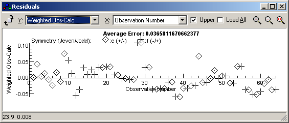
Select the Y axis of the plot. Possible
choices are:
- Weighted Obs-Calc
- Unweighted Obs-Calc
- Weighted (Obs-Calc)/Obs = Relative weighted error
- Unweighted (Obs-Calc)/Obs = Relative unweighted error
- Observed
- Calculated
- Observed and Calculated
- Weight
The last 4 are not residuals, but can be useful for indicating the data
included in the fit
|
 |
Select the X axis of the plot. Possible
choices are:
- Observation Number
- Frequency
- State Energy (Use the "Upper" check box to select the lower
or upper state)
- Calculated value
- Observed Value
- Weight
- Population
- J
- N
- F
- A: Ω for linear molecules, |K| for symmetric tops, Ka for asymmetric tops
- B: F1, F2...for
linear molecules, Kl for
symmetric tops, Kc
for asymmetric tops
- F1 Hyperfine
quantum numbers (if appropriate)
- F2
- ...
- F9
|
 |
Check to use upper (rather than
lower) state quantum numbers or state energy.
|
 |
Plot data with zero weight
(which would otherwise not be plotted).
|
 |
Zoom into region selected with
mouse.
|
 |
Zoom plot out.
|
 |
Reset plot to fill window.
|
