| <Prev Next> |
Data file: so.pgo
This example reproduces the results of "Laser magnetic resonance
spectroscopy of SO in the X3Σ - state
with a CO2 laser as a source", K. Kawaguchi, C. Yamada
and E. Hirota, J. Chem. Phys. 71,
3338 (1979) and "Microwave spectrum of the SO radical", F. X.
Powell and D. R. Lide, Jr., J. Chem. Phys., 41, 1413 (1964). It provides a
good example of calculating the effects of external fields.
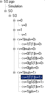
The later paper gives rotational constants for both v=0 and v=1 in the ground electronic state, and these are straightforward to enter, as described in Making a Linear Molecule Data File. In this B, λ, γ, DN and λN are available. Following the procedure will produce a simulation of the infra-red spectrum of the fundamental band of SO. Simulating the Zeeman or Stark effect is more complicated, and the complete data file has 3 Transition Moments objects with 9 individual Transition Moment objects beneath them, as summarized in the diagram:

The transition moments are made up
as follows:
The 32S18O
isotope has not been included in the data file, but could be by
duplicating the structure above. In principle the
<v=1|mu|v=0> Transition
Moments object could also have magnetic dipole components,
but these are likely to give much weaker transitions, and would
only be important in the absence of an electric dipole moment, as
in O2.
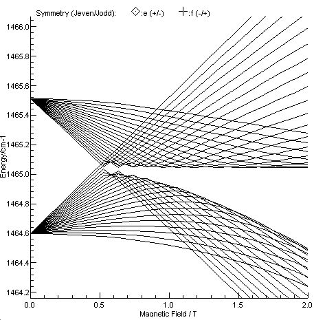
Figure 3 of Kawaguchi et al, showing the Zeeman effect in J = 20 and 22, N = 21 in v=1 is re-simulated
below.

To fit line position data in the presence of a field requires
the use of EField and BField directives in the input
file, typically immediately before before the affected lines.
For example, the data in Table 1 of Kawaguchi at al can be
used as follows:
LMR transitions; these are unusual in that the line position
is constant, but the field value varies. There are various
ways of specifying the data; taking the first transition in
the table as an example:
12C18O2 line R(34)
1104.91097 cm-1 N,J = 17,18 ←
18,18 MJ = 18 ← 18 Field = 3004
Right clicking on a simulated peak and copying the line from
the linelist window yields:
BField 0.3004
SO v=1  18  -  1 v=0  18  -  3    1104.91097 - 1.8e-7      0 : pQ12(18)18,18 : v=1 v=1 18 17 F1e 18 - v=0 v=0 18 18 F2f 18
The molecule need not be specified, as there is only one, and
manifolds will default to v=1 for the upper state and v = 0
for the lower state so this can be shortened to:
BField 0.3004
18 - 1 18 - 3 1104.91097 1
In this mode the text after the (relative) standard deviation
(here 1) is just taken as a comment, so can be omitted, and
the symmetry will be ignored in the presence of a field. Only
M and the eigenvalue number need to be specified.
The two input lines above require the eigenvalue numbers to
be known, which is tricky to work out from the data in the
table. Setting the eigenvalue numbers to zero means they will
be worked out from the transition label at the end of the
line:
BField 0.3004The quantum numbers at the end of the line are in order J N and M.
18 - 0 18 - 0 1104.91097 1 : v=1 v=1 18 17 F1e 18 - v=0 v=0 18 18 F2f 18
Alternatively branch format can be used:
BField 0.3004
pQ12(18),18,18 1104.91097 1
The branch is specified in the order:
BField 0.3004
pQ12(18)18,18 1104.91097 1
BField 0.3213
pQ12(18)17,17 1104.91097 1
BField 0.3751
pQ12(18)15,15 1104.91097 1
BField 0.4105
pQ12(18)14,14 1104.91097 1
The last block of data points in the table are also worth commenting on, as these correspond to microwave, rather than infra-red transitions. The field free transitions in v=1 can be input with
ScaleStdDev 0.1Note:
LowerManifold v=1
BField 0
pR1(0) 0.99900 1
rR1(1) 2.09120 1
rQ32(1) 0.42537 1
rQ32(2) 1.18287 1
rQ32(3) 2.16164 1
Finally the v=0 microwave transitions can be input with:
LowerManifold v=0
UpperManifold v=0

BField 0.57433
pR1(0)-1,0 0.83165 1

BField 0.72408
rQ32(2)2,2 0.83078 1
BField 0.80262
rQ32(2)1,2 0.83064 1
BField 0.83331
rQ32(2)2,1 0.83087 1