 Procedures
| Procedures
|
<Prev Next> |
The effect of a static external
electric and/or magnetic field can
be included in PGOPHER
simulations. Setting up a data file in principle only requires making
sure the required electric or magnetic dipole moments for the state(s)
of interest
are present. As the underlying physical interaction is the same as
absorption or emission of radiation, these are set as transition
moments. The only difference in the treatment of static fields is that
only transition moments acting within a manifold are considered. For
sample data files see:
The
presence of a
static field has significant consequences for the way calculations are
performed, and the way various windows work.
To simulate a spectra in the presence of a field, just set EField
and/or BField as required in the Simulation object
using the Constants window but note:
The only good quantum number in the
presence of a field is the
projection of the total angular momentum along the field, M, so the basis used for any one
diagonalization includes all states with the required M. The M quantum number will be added onto
the end of any other quantum numbers in the state and basis labels. As
this is a notionally infinite
number of states, the range for the total angular momentum included in
the
basis is taken from Jmin to Jmax.
(All rovibronic symmetries are included in the
same matrix.) A full matrix diagonalization is used, not a perturbation
based approach which is also in common use. The results will be exact,
provided a large enough range of total angular momentum is used, though
possibly slow.
The slow speed arises because the matrices to be diagonalized are much larger matrix than for zero field calculations. This can be mitigated by choosing Jmax (and possibly Jmin) carefully. The range must not be set too small as it controls the accuracy of the calculations. As a rule of thumb a range including total angular momentum one higher and one lower than the states of interest will typically give the correct trends, and the convergence of the calculations should be checked with respect to increasing the range.
The resulting file is available as
symstark.pgo.
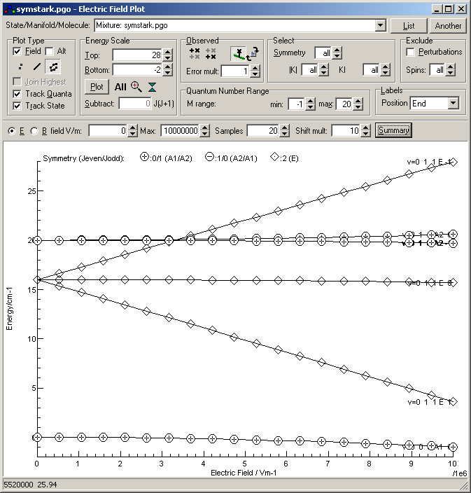
Note that the J = 0 level show a small, quadratic (second order) effect, while the K = 1 levels show a strong linear (first order) splitting.
Two levels of detail are available from this window. The "List" button prints out the energy levels as a function of field, as for example:Energy Level List for symstark.pgo
M Sym # Field(V/m) Energy g Population Name J K (kl) Sym M
0 - 1 100 -0.0000 1 .675473722 v=0 0 0 A1 0
0 - 1 1000000 -0.0010 1 .675569751 v=0 0 0 A1 0
0 - 1 2000000 -0.0040 1 .675857881 v=0 0 0 A1 0
0 - 1 3000000 -0.0089 1 .676338232 v=0 0 0 A1 0
0 - 1 4000000 -0.0158 1 .677011004 v=0 0 0 A1 0
0 - 1 5000000 -0.0247 1 .677876479 v=0 0 0 A1 0
0 - 1 6000000 -0.0355 1 .678935021 v=0 0 0 A1 0
0 - 1 7000000 -0.0483 1 .680187072 v=0 0 0 A1 0
0 - 1 8000000 -0.0631 1 .681633159 v=0 0 0 A1 0
0 - 1 9000000 -0.0798 1 .683273889 v=0 0 0 A1 0
0 - 1 10000000 -0.0985 1 .685109954 v=0 0 0 A1 0
Linear: -9.85038087317928E-009 cm-1/(Vm-1) -.0586611 Debye (15%)
Quadratic: -9.84803161106173E-016 cm-1/(Vm-1)^2 (.061%)
The values shown here are for the J
= 0, K = 0, M = 0 level, as can be seen from
the state label at the end of the line. To provide a simple model for
the behavior, a least squares fit is performed of energy against field
to the following three functions:
| E(F) = E0 + CF |
Linear, corresponding to a first order stark effect |
| E(F) = E0 + cF2 | Quadratic, corresponding to a second order stark effect |
| E(F) = E0 ± (Δ2/4 + C2F2)½ | Two level model giving intermediate behavior. It corresponds to two levels at E0 ± ½Δ, mixed by a matrix element CF. The sign of the square root is taken to be the same sign as C. |
In the above, F is the
field, E(F) is the energy as a function of
field, E0 is the
energy at zero
field (except in the last case where it is E0
± ½Δ) and c, C and Δ are constants. PGOPHER performs a fit to all
three functions for each level, though the results for the two level
model are not displayed if the fit gives poor results, typically when
the state is close to pure quadratic behavior. The %ages
indicate the maximum error in energy from the fitted function as a
percentage of the total energy change over the sweep. For the values
given above, the error in the quadratic fit is thus 0.061% of 0.0985 =
0.00006 cm-1, while the maximum error in the linear fit is 15% of
0.0985 = 0.015 cm-1, so the level clearly has a second order Stark
effect.
The J = 1, K= 1, M = 1 level is a classic example of a linear Stark effect:
   1    -   1 100             16.0000    1 .067584303 v=0  1  1 E  1
   1    -   1 1000000         15.8780    1 .068780609 v=0  1  1 E  1
   1    -   1 2000000         15.7556    1 .070002665 v=0  1  1 E  1
   1    -   1 3000000         15.6328    1 .071250937 v=0  1  1 E  1
   1    -   1 4000000         15.5095    1 .072526022 v=0  1  1 E  1
   1    -   1 5000000         15.3858    1 .073828535 v=0  1  1 E  1
   1    -   1 6000000         15.2616    1 .075159102 v=0  1  1 E  1
   1    -   1 7000000         15.1371    1 .076518368 v=0  1  1 E  1
   1    -   1 8000000         15.0121    1 .07790699  v=0  1  1 E  1
   1    -   1 9000000         14.8866    1 .079325643 v=0  1  1 E  1
   1    -   1 10000000        14.7608    1 .080775017 v=0  1  1 E  1
Linear: -1.23923698142084E-007 cm-1/(Vm-1) -.7379921 Debye (.262%)
Quadratic: -1.15112688486556E-014 cm-1/(Vm-1)^2 (17.2%)
Two Level:  16.004875 cm-1  .00993999 cm-1 -1.24153225238959E-007 cm-1/(Vm-1)  -.739359  Debye (.209%)
The linear fit is clearly better than
quadratic here, though a small
amount of second order behavior is also suggested by the slightly
better fit to a two level model. For the
linear and two level cases C
can be considered as an effective (state dependent dipole moment); the
textbook formula for the linear Stark shift in a symmetric top is
MK/(J(J+1))
·
μF giving an
effective dipole of MK/(J(J+1))
·
μ
=
1.1/(1.2)
·
1.45 = 0.725 Debye, with the 0.738
value resulting from higher order effects.
The "Summary" button prints out a summary of the fits for each level:
M Sym # g Population Name J K (kl) Sym M Energy Linear Dipole Err Quadratic Err Two Level Delta C Dipole2 ErrSee The pure rotational spectrum of the ground state of NH3 and the Stark effect for an example that is between first and second order.
-1 - 1 1 .067584122 v=0 1 1 E -1 16.0000 1.1947733e-7 .71151304 .304% 1.11179096e-14 18.5%
-1 - 2 1 .038010557 v=0 1 0 A2 -1 20.0000 -2.96324193e-9 -.0176467 15.8% -2.963163e-16 .008%
0 - 1 1 .675473722 v=0 0 0 A1 0 -0.0000 -9.85124183e-9 -.0586663 15.8% -9.8490399e-16 .071%
0 - 2 1 .067584185 v=0 1 1 E 0 16.0000 -2.96324193e-9 -.0176467 15.8% -2.963163e-16 .008%
0 - 3 1 .038010557 v=0 1 0 A2 0 20.0000 5.898223888e-9 .03512518 15.8% 5.89597675e-16 .121%
1 - 1 1 .067584247 v=0 1 1 E 1 16.0000 -1.23924255e-7 -.7379954 .276% -1.1562606e-14 17.8% 16.004337 .00918344 -1.24055462e-7 -.7387768 .244%
1 - 2 1 .038010557 v=0 1 0 A2 1 20.0000 -2.96324193e-9 -.0176467 15.8% -2.963163e-16 .008%