Procedures Automatic Fitting

<Prev Next>

Automatic Fitting of an N₂O IR Spectrum

This walk through shows how to use the automatic assignment process on the N₂O sample file provided in the Walk-through of Simulating and Fitting a Simple Spectrum (which this assumes you are familiar with). This is perhaps too simple an example to use automatic fitting on, as the assignment is fairly obvious, but it does demonstrate the procedure. The process described here is general, and could in principle work on any type of molecule or spectrum that PGOPHER could simulate. See also the following walk through, which uses the enhanced diagnostic tools that will not necessarily be useful in all circumstances. Note also that the many of the choices of peaks and values made below are arbitrary, and the walk through could have worked just as well with many other choices.

A. Generating the peak list

1. Load the overlay N2Onu2.ovr.
2. Right click on the overlay and select "Baseline and Peaks...".
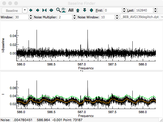
3. The first step is to determine a baseline. For this spectrum, the baseline is essentially flat, but has a small ripple, so use the zoom buttons to zoom in on a small sample of the spectrum to show the ripple. (The zoom buttons in this window work in the same way as the in the main window.)
   
4. Press the "Smooth" button to calculate a baseline. The orange line shows the calculated baseline, and the green line indicates the upper limit of the points used in calculating the baseline. The upper pane shows the spectrum after subtracting the baseline. The expand vertical button () can be helpful in expanding the baseline. Experiment with the "Window", "Noise Multiplier", and possibly the "Noise Window" settings and with "Dense" selected . You need to click on the "Smooth" button after changing the settings to update the display. The algorithm used by the "Smooth"  button works by attempting to identify points on the baseline (within the noise multiplier) and taking a moving average over the window. A "Window" of 30, "Noise Multiplier" of 2 and selecting "Dense" gives good results for this spectrum:

   
5. If you want to save the spectrum with the baseline subtracted, select "Make New" under "Make Overlay" to generate an overlay with a flat baseline.
6. To make a line list, adjust the "Noise Multiplier" so that the green line is above almost all of the noise. It is not necessarily the same as used for the baseline calculation - in this case a "Noise Multiplier" of 3 is promising. Selecting "Live update" will show the lines found in the upper window in blue automatically as the parameters are changed, though note this can be slow if the selected region is large. A minimum width and area can be selected; for the current spectrum the "Min Width" is too large, so deselect it, or change the value.
   
7. When you are happy with the result, generate the line list by pressing "Peak Find" and then "Make New" under "Make Line List". The resulting line list will be added to the overlays, and show in the main window.
8. In the current example, the above settings give bad results for one or two regions where the noise is larger, so re-run the peak finder over smaller regions as follows:
1. Select the region to update by either:
   

   1. Zoom to the region in the baseline window
   2. Make this the active region for peak finding pressing "Visible Here" on the right.

   or:
1. Select a region in the main window, and zoom the main window to that region
   
2. Make this the active region for peak finding by pressing "Visible in Main" in the baseline window.
   
2. Adjust the noise multiplier (or other setting) as required.
3. To replace the peaks in the line list, press "Peak Find" then "Append" under "Make Line List", making sure the generated line list is selected and "Erase Current Region" is checked when prompted.
4. Repeat as required - to reset the window, press the "All" button in the right (not the top) of the baseline window.
9. To delete individual lines from the line list in the main window, right click on the line and select "Delete Point"
10. To delete several adjacent lines, select them (left click and drag) and then right click and select "Delete Points".
11. To add individual lines by manual measurement, right click and drag over the peak in the baseline window.
12. The original experimental spectrum is not required at this point - you may want to hide or remove it from the main window by right clicking on it and selecting the appropriate option. You may want to use it later, though, for checking for weak peaks that the automatic peak finder may have missed.
13. The line list is saved as N2Onu2lin.ovr, using "Save Overlay As...".

B. Basic Automatic Fit Operation

1. Setting up the automatic fit

1. Set up an approximate simulation, and select the parameters to be determined.
   
1. Generate the basic molecule type with "File", "New", "Linear molecule" and set the excited state Lambda = Pi.
2. Manually adjust the origin, and upper and lower state rotational constants to produce something that is qualitatively correct. The simulation does not have to be that good - see the discussion of the search window below. The description below uses B"= 0.45, B' = 0.451, excited state Origin = 588.7 cm^-1.
3. The parameters to be determined, here origin, B' and B" should have "Float" = yes. At this stage the absolute minimum of parameters should be floated.
   
2. Select the transitions for trial assignments and fitting, the "fit" transitions. These need to satisfy the following criteria:
   • The number should match the number of parameters marked as floating. (An excess number can be given, but this will dramatically increase the search time.)
   • The transitions selected should be sufficient to determine the parameters floated
   • The transitions should be clear in the experimental spectrum. This necessarily can't be known at the start of the process (as the assignments are not known), and is one of the reasons it might well be necessary to try more than one starting point. In general the simulation can indicate the strongest lines that are clear of other lines. In the current case the simulation suggests the central Q branch region should be avoided.
     

   For this case three transitions are required:
   
1. Right click on (say) one P and two R branch lines. (Selecting three lines in one branch will give a poor determination of the difference between the two constants.) The three transitions will appear in the line list window.
2. In the line list window, select "More, Advanced" to make the autofit options visible.
3. Click and drag the mouse to select the three transitions, right click and select "Mark for Autofit". A bold F will appear in the "Std Dev" column, and filled triangles will indicate their position in the main plot window.
3. Select the check transitions. The choice of these is less critical than the fit transitions, as not all of them need to be assigned as part of the autofit, but they again should be transitions with a good chance of appearing clearly in the experimental spectrum. In the current case a few P and R branch transitions would be appropriate
   
1.  Right click on (say) two R and two P branch transitions, so they appear in the line list window.
   
2. Click and drag in the line list window to select these transitions, right click and select "Mark as Check". A bold C will appear in the "Std Dev" column, and open triangles will indicate their position in the main plot window.
4. At this stage, your desktop should look something like this:
   
5. Decide on the controlling parameters for the autofit. There are two key settings:
1. The acceptance window, which is the maximum error expected for the check transitions after the trial fit. This is set in the box labelled "Accept" in the line list window. For the purposes of this walk-through we will leave this at the default (0.1), though in general a number of the order of the line width  (here 0.001) is more appropriate.
2. The search window, which controls how far each side of the initial "fit" line positions you want to search. The intent is that the approximate initial simulation should predict the "fit" transitions to be out by no more than this value. For this example 3 cm^-1 might be a good value. The search time will increase rapidly as this is increased, so in more complex cases the range may need to be considered carefully. It is set in the autofit window, which is brought up with "Overlays, Autofit...". The Test button in this autofit window will display the number of trials in the box at the top, and display some additional information in the log window.
   
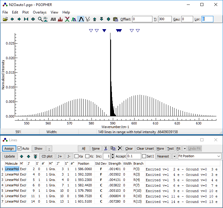
6. We are now in a position to try an autofit. The file saved at this stage (before the autofit) is available as N2Oauto1.pgo.

2. Using the automatic fit results

1. Press "Search" in the autofit window- after a short while, the window will list, for the best fits found:
   • nOK - the number of check transitions within the "Accept" window
   • Residual - the RMS observed - calculated for these check transitions.
   • SumI - the sum of observed intensity for these check transitions.
   • The values of the constants obtained for each fit.
   • Trial - The number of the trial. (This is typically only useful for debugging purposes.)
     
   • nDiff - the number of transitions different to the selected fit. This is only displayed if one of the fits is selected.

   Some additional information is shown in the log window.
2. To try out an individual fit, double click on that row. This will update the line list window with all the assignments made by that fit, and update the main plot with a simulation using these parameters. The standard residuals window will be shown. To try a different one, double click on that row; all the assignments and parameters will be updated. The Reset button will remove any assignments made by the autofit, and reset the parameters to their initial values.
3. The MinCheck setting deserves special consideration, as it determines the trials displayed. The trials are sorted by nOK and then SumI, with the best fit at the top. If MinCheck is not zero this sort order is modified; the intent is that it can indicate how many check transitions are likely not to be found. If it is set to a positive value then the nOK is ignored for sorting, provided it is greater than or equal to MinCheck. A negative value has the same effect, but the threshold is the number of check transitions + MinCheck. The default of -1 implies trials with 0 or 1 unsatisfied check transitions are sorted together. MinCheck can be changed without re-running the autofit, and the displayed trials will update accordingly. For the current case, a value of -1 is allowing too many failed check transitions, and a value of 0 is more appropriate.
   
4. For the current case several of the trial fits with nOK = 4 look good, reflecting the fact that the P and R branch lines are approximately equally.01 spaced, and several fits with the same pattern of assignments but with all the J values shifted by the same amount will give good fits. For this particular spectrum, the best diagnostic is in fact the position of the Q branch - for the auto fit run exactly as above only fit number 4 has the Q branch origin in the right place. (It requires MinCheck = 0 to display.)
5. If none of the trials look good, and you want to re-run the autofit with different settings, the Reset button will remove any assignments made by the autofit, and reset the parameters to their initial values.
   

3. Specifying possible ranges for parameters

While the above process has produced the correct assignment as one of the possible trials, it is not obvious from the list presented. The autofit can be made more selective by specifying allowed ranges for one or more of the parameters to be determined. This can also speed up the search, as trials are discarded more quickly. For example, for the spectrum given here the manual estimate of the band origin is likely to be within 0.5 cm^-1 of the actual value. To re-run the search above with this constraint:

1. If you have not done so already, press the Reset button to discard the autofit assignments
   
2. To limit the range of a particular parameter, set the maximum permitted change (+ or -) as the "Std Dev" for the parameter in the constants window. In this case set "Std Dev" for the excited state origin to 0.5. Tip: this should be blank if you don't want to apply a constraint; before autofitting make sure that the standard deviations of all unconstrained floated parameters are blank, and don't have standard deviations from previous fits present. (Click on the down arrow in the autofit window and select "Clear Parameter Ranges" to do this.)
   

1. Press the Reset button to discard the autofit.
2. Set "Std Dev" for B in both the ground and excited state to 0.05.
   

C. Adding More Lines

1. Adding lines that are now (more or less) correctly simulated

1. Now add some more candidate lines for assignment in the region:
1. Open the transitions window "View, Transitions", and select some lines, say the P and R branch lines by setting "Change" to "<>", implying not equal. Some additional selectivity can help - click on "Filter" to make some extra options available. The options available are:
• "In Plot Range" which discards lines outside the main window plot range.
• "Strength" which discards lines less than a fraction of the strongest (10% by default).
  
• "Discard Duplicates" (enabled by default) which makes sure lines already in the line list window are not duplicated.
2. When you are happy with the selection displayed click "Add". This will add entries to the line list window for all the transitions selected by the window.
   
2. The expectation is that at this stage many lines will be simulated in approximately the right place. There are two possible approaches to take, either just taking the nearest (typically the easiest):
   
   1. Select all lines in the line list window (Press All).
   2. Press the "Nearest" button in the line list window, which simply assigns each unassigned line to the nearest line within the acceptance window.
      
   or a modified autofit:
   1. Select all lines in the line list window (Press All).
   2. Mark all the lines as search transitions (right click and select "Mark for Autofit".
      
   3. In the autofit window, reduce the search window to, say, the same as the acceptance window in the line list window, or something close to the average error in the current fit. In this case, try 0.01. (The file at this stage is saved as N2Oauto3.pgo.).
   4. "Search" will now try all unassigned lines close to the predicted lines; this should be quick, provided the window is set small enough. The search in this case will typically fail for some lines, in which case only one or two candidate sets of assignments are produced:
   • The upper row takes the closest observed line to each prediction provided the observed line is within the search window.
   • The lower row simply takes the closest line to each prediction, regardless of how far out the prediction is. This is omitted if it would be identical to the upper row.
   In the current case, either produces method gives good results, so we proceed assuming the "Nearest" method has been used. The file at this stage is saved as N2Oauto4.pgo.

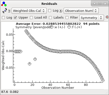
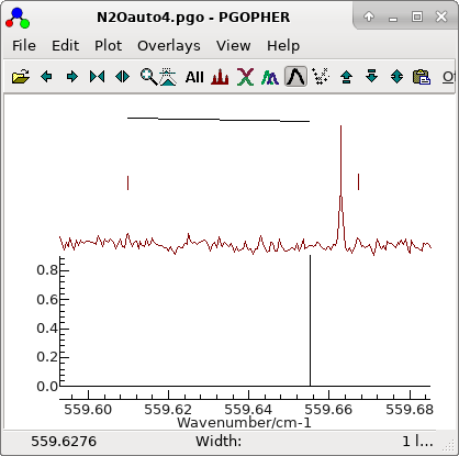
2. Adjusting assignments using the residuals window

1. The residuals window shows essentially a regular pattern, with some glitches:
   

   
   

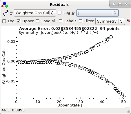
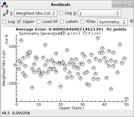
   This plot makes more sense if plotted against J, rather than observation number:
   

   
   
2. A fit suggests there are two mis-assigned lines:
   

   
3. To fix the mis-assignment right click on one of the points in the observations window and try one of the following:
1. Select "Show and Edit". This will highlight the relevant observation in the line list window, and centre the plot on the transition. (This is most useful if the "Expand" button () is pressed a few times so the window only shows a small plot range.)
   

   
   

   Here, the wrong choice of line has been made; right clicking and dragging across the strong line will update the assignment to the correct value. At this stage, consider checking suspect or missing lines against the original spectrum, rather than the line list.
2. The quick fix (... to sweep it under the carpet) is simply to select Clear Point(s)" on right clicking on the suspect point in the residuals window. This will set the "Std Dev" to 0 for the transition, excluding it from the fit.
   
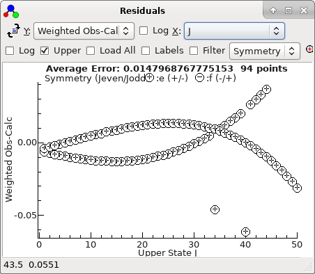
4. With the two bad points removed, the residuals look good, and can be much improved by floating D in both states. refitting gives a good set of residuals saved as N2Oauto5.pgo.) The residuals now look entirely random:
   

   
   
5. To scan for additional assignments after fitting, on the assumption that some calculated lines will have moved into the acceptance window:
1. Update the calculated positions selecting all the lines in the line window and pressing "Update". This will change the calculated frequency and intensity of unassigned lines.
2. Press the "Nearest" button. (In this case it will assign the two peaks removed above.)
   
3. Fit as usual to refine the parameters

D. Determining additional parameter(s) - the Q branch

In the current case the Q branch is not simulated, and it needs the determination of an independent parameter (q). Again this case is sufficiently straightforward that the assignment could be done manually, but the autofit process is demonstrated here also. As a single parameter is to be determined, a single trial fit transition is required, yielding a very quick search. A possible process is as follows:

1. Zoom in to the very start of the Q branch, and right click on a few transitions to add them to the line list window.
2. Select one of these as the trial fit transition, and the rest as check transitions.
3. In the constants window, float q in the upper state.
4. Make sure all all the standard deviations are blank ("Fix", "Clear All Std Dev...", "Mixture" in the constants window) otherwise they will act as constraints on the search.
5. A much smaller search window is needed - 0.2 cm^-1 should be plenty.
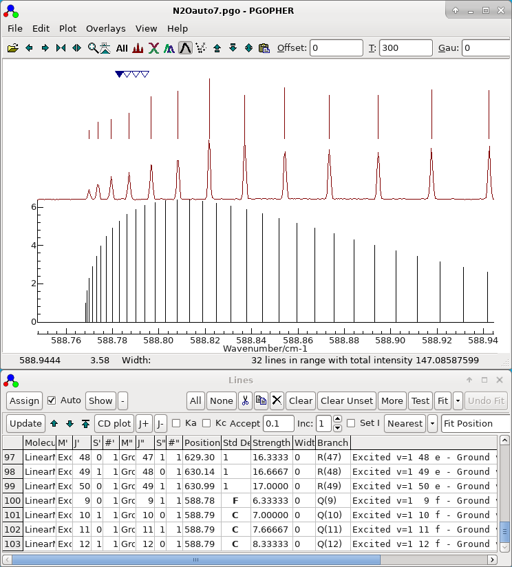
6. Note all the parameters determined so far are left floating, and all the observations assigned so far are left in the autofit process. The file set up for autofit in this way is saved as N2Oauto7.pgo and the display should look something like this:
   
   
7. In this case the top fit is much better than the others. The process described in the previous section under "Adding More Lines" can then be used to assign the remainder of the transitions. In the transitions window use set "Change" to Q) and the "Nearest" button will assign almost all of the transitions. After adjusting one bad assignment, and allowing q_D to float yields the final result, N2Oauto8.pgo. The final fit yields:

SVD fit: 144 Observations,  7 Parameters (scaled)
Initial Average Error: 0.0000586651493283788
Predicted New Error:   0.0000586651493283779
Parameters:
  # Old                 New                 Std Dev   Change/Std Sens    Summary              Name
  1 .4190113492580969   .4190113492579454   2.8034e-7    0.0000  7.7e-10 0.419011349(280)     Ground v=0 B
  2 1.76173067092025e-7 1.76173067018370e-7 9.963e-11    0.0000  4.2e-13 1.761731(996)e-7     Ground v=0 D
  3 588.7679935134044   588.7679935134028   9.3805e-6    0.0000  8.38e-7 588.7679935(94)      Excited v=1 Origin
  4 .4195742866345234   .4195742866343714   2.7720e-7    0.0000  7.6e-10 0.419574287(277)     Excited v=1 B
  5 -.00079196442418883 -.00079196442412925 3.2019e-8    0.0000  1.52e-9 -7.91964(32)e-4      Excited v=1 q
  6 1.78921147979445e-7 1.78921147906146e-7 9.669e-11    0.0000  4.1e-13 1.789211(967)e-7     Excited v=1 D
  7 9.9216205147776e-10 9.9216201696816e-10 1.759e-11    0.0000  8.2e-13 9.92(18)e-10         Excited v=1 qD

Correlation Matrix
Largest off-diagonal element = 0.996 at 4,1 = Excited v=1 B, Ground v=0 B
       1       2       3       4       5       6       7
  1   1.000
  2   0.912   1.000
  3   0.102   0.135   1.000
  4   0.996   0.901   0.039   1.000
  5  -0.151  -0.220  -0.060  -0.161   1.000
  6   0.914   0.994   0.072   0.912  -0.234   1.000
  7   0.209   0.307   0.084   0.214  -0.954   0.316   1.000