Walk-through of Simulating and Fitting a Simple Spectrum
Note: Clicking on the links to files below
may (depending on the browser) show you the file contents as xml;
to download the files right click on the link and select "Save
Link Target As...".
This section walks through the typical steps that
might be used for working on a spectrum. The example chosen is the
infra-red spectrum of the bending vibration (ν2) of
N2O, but the steps shown here are not specific to this
spectrum. The file N2Onu2.ovr
(right click the link and select "Save Link Target As..."
to download the file) is provided for you to work through the
steps in the analysis, which are:
- Loading the spectrum and setting up a basic simulation
- Assigning and fitting the spectrum
- Tools for understanding the spectrum - Fortrat plots and
Energy Level plots.
- Adding a microwave spectrum.
- Using and fitting to an external (JPL) line list
- Fitting to data from multiple sources
- More advanced fitting - hot bands
- Band contour Fits
- Adding custom parameters - the "other" hot band
- Using HITRAN data
Steps 1 to 3 provide a basic introduction, with the following
sections introducing more advanced features.
The spectrum provided is at a particularly high
resolution spectrum (0.001 cm-1). The high resolution
arises as the spectrum was taken on the far IR beam line of the Canadian Light Source and
was provided by Brant Billinghurst; the file size has actually
been reduced by a factor of 4 by averaging over 0.0005 cm-1.
The spectrum, and this walk-through were prepared as part of a
workshop on "Synchrotron Based Far Infra-red Vibrational
Rotational Spectroscopy" organised by Brant Billinghurst and the Canadian Light Source on
26-27 June 2015.
1. Loading the spectrum and setting up a basic simulation
Loading and Viewing the Spectrum
To view the spectrum, start the PGOPHER
program and drag and drop the N2Onu2.ovr
file onto the PGOPHER window (or use "File", "Load
Overlay…"). To view selected parts of the spectrum, select
the required portion with the mouse and press the zoom to selected
( )
button. The other key controls are:
 |
Simulate Spectrum |
 |
Compress plot to show all lines – use
this if no spectrum is visible or you are lost |
 
|
Pan plot left or right
|

|
Compress Plot
|

|
Expand plot
|

|
Cycle through various plot styles.
|
The spectrum shows the the classic P, Q and R branch structure
associated with a perpendicular band of a linear molecule:
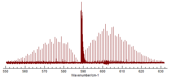
To simulate this, select "File", "New", Linear
Molecule". This gives a simulation of the rotational structure of
a vibrational transition of a linear molecule with rotational
constant 1 cm-1 and band origin (≈ vibrational
frequency) 1000 cm-1, placed below the experimental
spectrum. To start with we will just look at the P and R branches
and ignore the Q branch (the strong central feature). This means
the energy level formula is very simple:
E(J) = Origin + BJ(J+1)
to which we will consider adding centrifugal
distortion terms −DJ2(J+1)2
+ HJ4(J+1)4, though they are
not essential for this exercise.
Saving Files
This would be a good point to start saving files.
Note that, when saving, the experimental overlay and simulation
parameters are saved in separate files. Simply using
“File”, “Save” will save a .pgo file that
only contains (at this point) the rotational constants and band
origin. Later on it will contain some assignments. To save the
overlay (if required) use “File”, “Save
Overlay”, though it is often easier to reload from the
original file.
Manual Adjustment of Parameters
To adjust the constants the program uses select
"View", "Constants" which brings up the Constants Window. The most obvious
thing to adjust is the band origin (approximately the band centre)
to place the band in about the right place. Click on the v=1
entry under Excited and set Origin to 590.
Press the simulate ( ) button to update the simulation and use
the zoom to selected (
 ) button to just display the band of
interest.
The next obvious thing to adjust is the band type
- the default spectrum is missing the central Q branch. This is
fixed by setting the upper vibrational state symmetry to Π, as
it has one quantum of the bending vibration. Click on the v=1
entry under Excited and set Lambda to Pi
and re-simulate. This will introduce the Q branch to the spectrum:
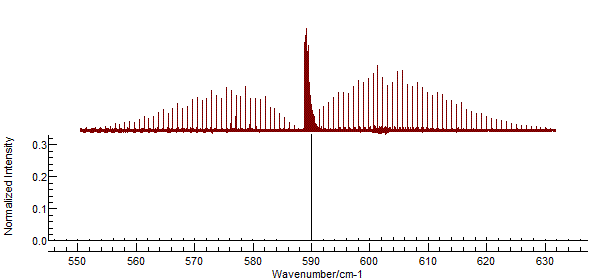
The strong central Q branch has adjusted the
scale so that the features to the left and right almost disappear.
This is an artefact of the default parameters, which make the
(unrealistic) assumption that the rotational constants are the
same in both states. To investigate try making small adjustments
to the B value in the upper state (underneath the Origin).
Mouse Adjustment of Parameters
This is a good application of the mouse adjust
function – right click on B and select Turn
on Mouse Adjust, after which the mouse wheel will step the
rotational constant. You can click on different parameters to
switch the adjustment to these; the "active" parameter is shown in
bold. Hitting "Esc" stops the process and resets the value; using
the menu will also stop the process but leave the adjusted value.
If the default step size is too small or too big you can manually
set the step size by entering a number under
“Increment”. This mode can be confusing if left on, so
remember to turn it off before the next stage.
2. Assigning and Fitting the Spectrum
Estimating the Rotational Constant
To improve the simulation requires more precise
values of the rotational constants, B, for the upper and
lower states. We could legitimately obtain these from the
literature or ab initio calculations of the geometry, but
for the purposes of the current exercise we will determine them
from the spectrum. Try improving the simulation by manually
adjusting B for the upper and lower states. To set the
lower state rotational constant click on the v=0 entry
under Ground. As a tip, the two rotational constants
should be about equal, though not exactly to avoid issues with the
central Q branch. (This dual adjustment is best not done with the
mouse adjustment function.) The aim of this step is to be able to
adjust the simulation until you can make a reasonable guess for
the assignments of the lines, i.e. which line in the
simulation corresponds to which line in the experimental
spectrum. This is best started with the low J lines around
the band origin.
In the current case, setting rotational constants to about 0.5 cm-1
gives promising results as shown below. Possible assignments are
indicated in blue.
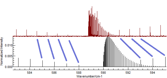
(This plot is obtained with
B'
(Excited state
B) = 0.502, and
B" = 0.5, and
zooming in to the central part of the spectrum.)
Line Position Assigning
The next step is produce a list of experimental line positions
and the quantum numbers for the transition. When following the
steps below, expect to have to make some corrections; the
program is designed to make mistakes easy to detect and correct.
- Right click on one of the peaks in the simulated (lower)
spectrum that you think you can assign. A Line List Window will appear:

You will normally want to arrange the windows so that the
simulation and the line list do not overlap. Selecting View,
Arrange Windows from the main menu may help.
- All the lines close to the mouse (within a few pixels on the
screen) will be shown selected, which will often catch more
than one rotational transition. The intensity of the
individual transitions (shown under Strength) is normally
enough to indicate if you have a sensible selection of lines.
The next step will ignore the weaker lines, or you can adjust
the selected lines with the mouse. You can delete the unwanted
transitions by selecting the required rows with the mouse and
pressing the delete button,
 .
.
- Measure the corresponding peak in the experimental spectrum
by dragging the across the peak with the right mouse button.
(Press and hold with the right mouse button to the left of the
peak, drag the mouse to the right of the peak, and release).
The peak position will be determined from the spectrum and a
marker indicating the determined position will be displayed.
Note:
- The exact positions you click and release on in the
experimental spectrum is not important, provided you do not
include any other peak in the range. For closely spaced
peaks you may need to try more than once, possibly expanding
the scale.
- You can remove the markers from the simulation from the
Overlays menu - select "Delete Last Peak" or "Clear All
Peaks" as required.
- Provided Auto is
selected in the line list window, the "Position" column in the
line window of the selected rows will change to the measured
position of the experimental peak and the “Std
Dev” column will be set to 1 to indicate a measured,
rather than a calculated frequency. (If Auto is off press the
Assign button to do
this manually.)
- Repeat steps 1 to 4 to assign a few more peaks.
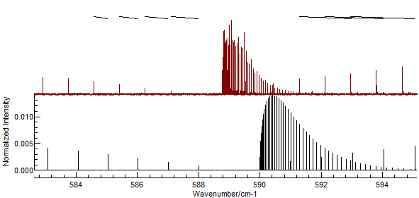
- To check that you have the correct assignments, press the
"Test" button. The program will read and plot your
assignments:
- The observed and calculated values are joined with lines
above the experimental spectrum.
- The upper end of the line is the experimental frequency,
and the lower end is the calculated frequency.
- When the fit is perfect, these will appear as small
vertical tick marks. At this stage the lines will probably
be sloping, but it is normally obvious if you have
miss-assigned something.
- Positioning the mouse over the top of one of the marks
will show the number in the line list of the assignment in
the status bar below the simulation.
- Right click on the mark to show the row containing the
experimental line position in the line list window.
If you enter the assignments indicated in the picture above, the
"Test" button should give a picture like this:
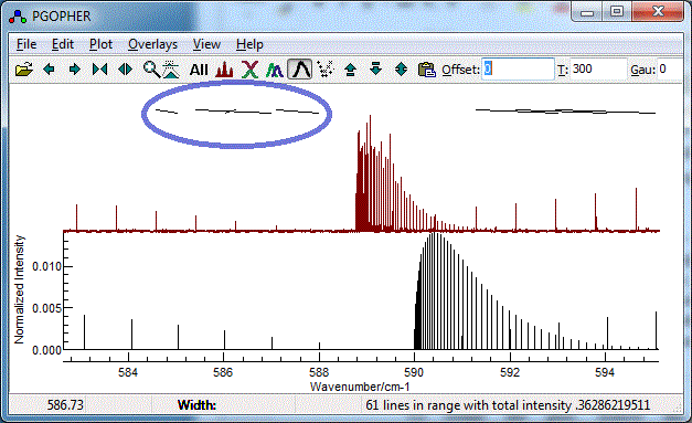
- It is easy to miss-assign peaks, and wrongly assigned peaks
can distort the subsequent fit quite badly An error might give
a plot such as:
To correct an assignment, select the corresponding rows(s)
with the mouse and either:
- Delete those rows with the delete button

- Re-measure the peaks as in step 5 by dragging across the
peak with the right mouse button.
- Manually edit the values in the grid. You can
temporarily remove an observation by setting the "Std Dev"
to zero.
Note that the assignments are saved in the .pgo file when
selecting File, Save along with updated constants.
Line Position Fitting
Given a reasonable number of assigned peaks you
can perform a fit. At this stage only a few assignments are
needed, and the fitting process will start by only trying to
determine correspondingly few parameters.
- Select the parameters you want to float by going to the constants window (View,
Constants) and set "Float" to "yes" by each of the parameters
you want to float, by clicking on "no". At this stage
appropriate constants to float are the upper and lower state
rotational constants, B and the origin of the upper
state.
- Click Fit in the line
list window.
- A list of observed and calculated transition frequencies,
the average overall error, new values for the constants and
estimates for their uncertainties and a correlation matrix
will be displayed in the log window
(View, Log though this will normally show automatically. You
will normally want to arrange your desktop so that the
simulation, line list and log windows do not overlap .) For
more details on the values displayed, see the documentation
for the log window.
- A plot of the residuals before the fit will be shown in the
residuals window. This is
normally shown automatically, or use View, Residuals.
- The main window will show an updated simulation.
- If the results look reasonable, then press the "Fit" button
(in the line list window, not the log window) repeatedly until
the error converges. Note that the residuals and calculated
positions displayed are the values before the fit, rather than
after.
- If the fit does not look good, the Undo Fit
 button in the log or line
list window; this will step constants back one fit cycle for
each press. Use this and consider:
- If you floated too many (or the wrong) parameters toggle
float as in step 2 and try again
- If you have some miss-assignments, see the previous section
for correcting them.
- If you are uncertain about some transitions - perhaps they
have poor signal to noise, or are blends of more than one line
- consider increasing the estimated relative error of the
peak. This is the "Std Dev" column; the defaut is 1,
but values of 3-10 are sensible for less clear lines. (Zero or
negative values exclude the peak from the fit entirely.)
Complete the fit by measuring up all the P and
R branch lines, or at least a reasonable selection of them. The
file at this stage is available as
N2Ostage1.pgo. For further
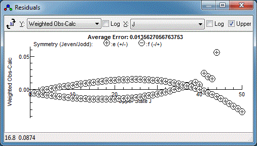
refinements of the fit the residuals window is most useful. With
all the P and R branch lines in it should look something like
this:
Note the choice of x axis made here
(the drop down in the top middle). The default is observation
number, but the J has been chosen for the plot above.
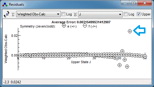
There is clearly a systematic trend in the residuals - perhaps the
centrifugal distortion constant, D, should be floated?
Floating both the upper and lower state D does indeed
improve the fit, but reveals a couple of lines are fitting
particularly poorly:
This is with my measurements - yours may well
look different. Any specific measurement can be checked by right
clicking on the point in the residuals window and selecting
"Show Transition". For best results the plot should be on quite an
expanded scale - if "Show Transition" has just been used the
expand plot button (

) will expand the plot about the
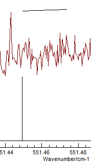
transition of interest. With the transition indicated with the
arrow above, the plot looks something like this:
It is clear from the top mark that I have been
careless in measuring this particular transition. To remeasure,
right click on the transition in the residuals window again, but
this time select "Edit Point". This selects the transition in the
line list window, and it can be measured again by right clicking
and dragging on the experimental spectrum. Repeating this for the
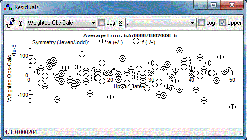
any other poorly fitting transitions and re-fitting should yield a
random set of residuals, which is a sign of a good fit:
3. Tools for understanding the spectrum
Various tools are available to understand the
simulated spectrum and the underlying pattern of energy levels.
Right clicking on an individual line will give the quantum numbers
associated with the line (or the strongest lines close to where
you click if there is more than one). The information is expressed
in more than one way; on the left hand side are the quantum
numbers always used internally, with extra information on the
right hand side. For a complete list see the
line list window documentation.
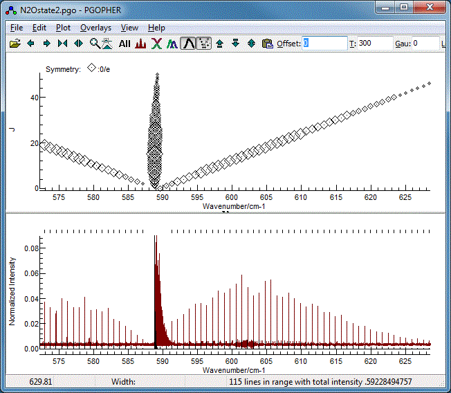
The Fortrat Diagram
The overall pattern can also be understood by turning on the
Fortrat plot with the Fortrat button( ). The
resulting plot has the same horizontal axis as the main plot,
but J as the vertical axis. This allows individual
branches to be picked out. A symbol is plotted for each
transition, and the size of the symbol proportional to the
intensity:
The Q Branch
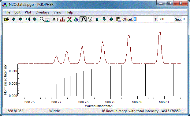
To finish the fit, we need to fit the central Q branch also.
Zooming in it is clear that, while the basic structure is
correct, the constants we have so far do not give the correct
spacing:
In fact we need to take account of the fact that the upper
state is degenerate, and consider l-doubling (known as
Λ-doubling if the degeneracy is electronic). The
upper state is a Π state, and thus doubly degenerate, with
two different parities for each J. The two different
parities have slightly different rotational constants, so the
energy level formula becomes:
E(J) = Origin + BJ(J+1)
± qJ(J+1)
If you now assign some of the Q branch lines and float q
(essentially the difference between the two rotational
constants) for the upper state, you should be able to fit the
entire spectrum. (Note that q for the lower state has no
effect, as the lower state has Σ symmetry and is not
degenerate.) The energy level plot should now show the splitting
in the upper state clearly. For a perfect fit you may need to
consider centrifugal distortion of q and float qD
and possibly the higher terms. Note:
- In the residual window, the Q branch will show as having a
different parity.
- The default highest J is 50, so you might need to
increase Jmax slightly to simulate all the
visible lines. This can be set at the state, manifold,
molecule or species level, and defaults to 50 at the species
level.
The file at this stage is available at
N2Ostage3.pgo.
Saving the Line List to a Separate File.
As a final step, save the list of assigned line positions in a
separate file; this allows more flexibility in fitting than is
available from the line list window, and will be important for
later. To do this, in the line list window click on "All" then
"More", "Save to File","In Simple Format...". For the purposes of
this exercise we will use the file name
N2OIRv1.obs. This produces a text
file, which is most conveniently edited with the
Tabslave Editor, distributed with
PGOPHER which has some special features to aid editing. (Any plain
text file editor could be used, though not word processors as they
can spoil the format.) The first few lines of the file are:
NQN 2
 1 e  2 e  587.09236   1  .00079  : N2O_0.001....dpt - N2Onu2.ovr
 2 e  3 e  586.25496   1  .00155  : N2O_0.001....dpt - N2Onu2.ovr
 3 e  4 e  585.41791   1  .00228  : N2O_0.001....dpt - N2Onu2.ovr
The first line, NQN 2 specifies the format of the following
lines. Each subsequent line has one observation with (in this
case) 7 items for each:
 J'p' J"p" Observed    σ  Comment
 1 e  2 e  587.09236   1  .00079  : N2O_0.001....dpt - N2Onu2.ovr
The first 4 items are the upper and lower state
quantum numbers, upper state first (p is the parity). This is
followed by the observed line position, and the estimated
(relative) error (σ). The rest of the line is taken as a
comment; the line list window has provided the calculated
intensity of the transition and the name of the file used for the
measurement (abbreviated in the above), but these can be omitted
or replaced if you are using an alternative method of generating
the line list. There are several other possible formats for line
lists - see Line List Input File Format
for more details. For example a "branch" type format is also
available; the above could also be saved as:
 P(2) 587.09236 1 .00079  : N2O_0.001....dpt - N2Onu2.ovr
 P(3) 586.25496 1 .00155  : N2O_0.001....dpt - N2Onu2.ovr
 P(4) 585.41791 1 .00228  : N2O_0.001....dpt - N2Onu2.ovr
Energy Level Diagrams
The underlying energy level diagram can also be
seen with "View", "Levels". The clearest plots are typically
obtained by plotting
E −
BeffJ(
J+1)
versus
J, rather than simply
E v.
J.
Beff
is chosen empirically to give the clearest plots, usually close to
the actual rotational constant. This "reduced" style of energy
level plot makes deviations from the overall trend clearer. It can
also plot the "observed" energy levels on the plot, calculated for
the upper levels by taking the calculated energy for the lower
levels and adding the observed energy, and vice-versa for the
lower levels. This can reveal trends in errors (suggesting
additional parameters are needed) and common difference failures.
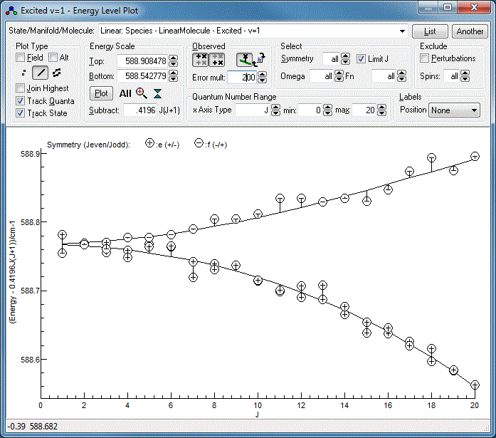
A good diagnostic for the current fit is obtained by:
- Setting "Subtract" to 0.42 cm−1 (or
whatever your B value is).
- Selecting "Linear: Species - LinearMolecule - Excited - v=1"
at the top to plot just the upper vibrational state.
- Clicking on the line style button,
 under
plot type, to show calculated energy levels as lines, rather
than symbols.
- Clicking on the "Observed" buttons,
 and
and  , to plot the "observed" energy levels.
- For the current fit the "observed" values are so close to
the calculated lines that the residual differences cannot be
appreciated. They can be magnified by setting "Error mult" -
try a value of 200 instead of the default of 1.
 and
and  , to
adjust the vertical scale. See the Energy
Level Window for further information.
4. Adding a Microwave Spectrum
Combining data from more than one source is
invaluable in improving the quality of fits. For the current
example microwave data is available, so we will make use of that.
The first step is to add the microwave spectrum to the simulation.
All that is required is to add the relevant dipole moment to the
model – the file constructed above only contains the v=1
– v=0 transition moment. The key steps are:
- Right click on “LinearMolecule”, and select
“Add New”, “Transition Moments”. In the
dialog you are presented with select “Ground” for
both Bra and Ket. This selects the manifold involved.
- Right click on the object created, <Ground|mu|Ground>,
and select “Add New”, “Spherical Transition
Moment”. This object contains the dipole moment –
the default value is 1 debye along the linear axis.
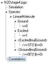
The tree of objects in the constants window (on
the left) should then look like this:
The
Simulation object contains
parameters controlling the simulation, such as linewidth and
temperature. The
Ground and
Excited objects
are
Manifolds, which contain one or
more
States (here
v=0 and
v=1).
Manifolds can be used to group states together, with the only
constraint on grouping that interacting states must be in the same
manifold. For the simulation here, both states could be in the
same manifold, though there is a slight speed advantage to keeping
them separate. Along with the manifolds,
Transition Moments objects
(here
<Excited|mu|Ground> and
<Ground|mu|Ground>)
contain one or more
Transition
Moment objects that link specific states. These are all
under the higher level
Molecule
object; additional molecule objects could be added for
isotopically substituted species, such as
15N
14NO
in this case. Additional
Species
objects could be added for completely unrelated molecules. For all
these items, duplicate names under any given object should be
avoided; they can be used when setting up the calculation in the
first place but should be renamed when possible.
Pressing Simulate and then All should reveal a new set of pure
rotational transitions at low frequency. In fact the microwave
transitions are rather weaker than the infra-red transitions so
they will not be visible on the same plot as the infra-red
transitions. Zooming the plot into the 0-50 cm-1
range should show them. As microwave transitions are usually
reported in frequency rather than wavenumber you may want to
switch the plot units to MHz – use “Plot”,
Units”, “MHz”. (Any simulation widths set will
automatically be converted, but note the line assignments
generated as above are not.)
5. Using and Fitting to an External (JPL) line list
Using a JPL Line List
A microwave line list is available from the JPL
spectral line catalogue at
http://spec.jpl.nasa.gov/.
Follow the “Catalog Directory with links” and look for
entry 44004. The file c044004.cat is the line list in text format,
and the first three lines look like:
Frequency/MHz FreqErr log10(I)DR   Elower gUP  Tag Qfmt Upper Qno   Lower Qno
   25123.2460  0.0004 -6.7155 3    0.0000  3 -440041303 1 0 0       0 0 0
   50246.3700  0.0130 -5.8150 3    0.8380  5 -440041303 2 0 0       1 0 0
   75369.2240  0.0100 -5.2911 3    2.5141  7 -440041303 3 0 0       2 0 0
The quantum numbers are J, l and
v. The file c044004edit.cat
has been edited to remove the IR and hot band transitions. (These
transitions are not normally included in JPL catalogue files. The
pdf link on the JPL site provides information on the file.)
PGOPHER can understand and make use of .par files in
various ways. To use it as a simple line list (i.e. as a list of
frequency, intensity pairs) load it as an overlay. (Tip: to load
at this point, without removing the previous overlay, right
click on the .cat file in a file explorer and select
“Copy” and then select “Overlays”,
“Paste Another” in PGOPHER. Alternatively
turn on “Merge” in the file menu before loading the
overlay, and then turn it off.) Note you might need to adjust
Jmax to reproduce the entire spectrum. This can be set at the
state, manifold, molecule or species level, and defaults to 50
at the species level.
The .cat files have absolute intensities, in
units of nm2 MHz. To force the experimental overlay to
use these units, make sure the intensity units in the Overlays
window ("View", "Overlays") are set to nm2MHzperMolecule
at both the top level and the c044004edit.cat object. To
make PGOPHER use the same units, set the same intensity
units in the Simulation object in the constants window.
For quantitative agreement on intensities, the dipole must be set
correctly. Helpfully this is provided in the JPL documentation
associated with the .cat file. The value (0.16083 D) should be
entered as the strength parameter in <v=0|T(I)|v=0>
in the constants window.
Fitting From a .cat Line List
The simulation and overlay of the microwave
should look fairly similar at this point, but can be improved by
using the line list for as input to a fit. This is (in principle)
easy for .cat files, as PGOPHER can (in principle) take
the assignments from the file without modification. To fit:
- Bring up the log window:
“View”, “Log”.
- Drag and drop the c044004edit.cat file to the log
window, or use the file open button (
 ) to
select the file via the standard dialog. Either will set the fit
file name in the top centre.
- Make sure the fit type in the top left is set to
“Line”
Fits should now work, though if you have been
following the complete instructions above you will need to fix
some now irrelevant parameters for sensible results. (The
“Undo Fit” button might be needed here and, in the
constants window, "Fix", "Fix All Parameters...", "Mixture".) The
residuals window is, as before, essential in tracking the progress
of the fit (“View”, “Residuals” if not
already visible). Note that c440004.cat contains a wide range of
observation weights (= standard deviation of the observations), so
you may want to set the plot to “Unweighted Obs-Calc”
to understand the fit in the early stages. It also contains a
mixture of calculated and observed line positions, and PGOPHER
will use only the observed line positions for fitting by default.
The file provided seems sufficient to determine
B,
D,
H and
L for the ground state. In addition to make
the text displayed in the log window useful you will need to
increase the precision of the displayed values - the
Precision setting at the top
level should be increased to 7 or 8. (Click on the
N2Ostage.pgo
at the top of the tree to set this.)
It is also possible to fit the dipole moment to the intensities
in the file. To do this:
- Fix all parameters floated in the previous fits
(“Fix…” in the constants window).
- Set the fit type (top left of the log window) to
“Intensity”.
- In the residuals window, use the reload button (
 )
to reload and recalculate the observations, and then fit if
things are set up correctly. For intensities plotting the ratio
(Calc/Obs in the top right) is typically more informative for
intensities than simply plotting Obs-Calc.
The file at this stage, after fitting ground
state rotational constants and dipole moment is available at
N2Ostage4.pgo.
6. Fitting using multiple sources of data
To produce a best overall fit, using both the infra-red and
microwave line positions, the lines are best placed in separate
text files. The line list window is convenient for getting
started in fitting, but for anything other than the simplest
fits a setup along the lines described below is much more
flexible. See List Input File Format
for full details of the format of the observation files.
From the instructions above, we have two files, N2OIRv1.obs. with the infra-red
data and c044004edit.cat.
To combine these we need a control file with the following
contents:
Colour Red
include N2OIRv1.obs
Colour Blue
include c044004edit.cat
Save this as N2Ocombined.obs and:
- Bring up the log window:
“View”, “Log”.
- Drag and drop the N2Ocombined.obs file to the log
window, or use the file open button (
 ) to
select the file via the standard dialog. Either will set the
fit file name in the top centre of the log window.
- Make sure all the parameters are fixed ("Fix", "Fix All
Parameters...", "Mixture")
- Make sure the fit type in the top left is set to
“Line”.
- In the residuals window, press the reload button (
 )
)
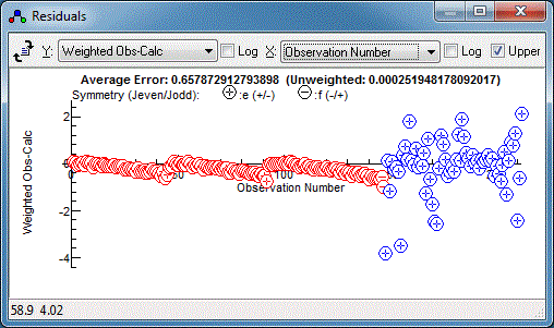
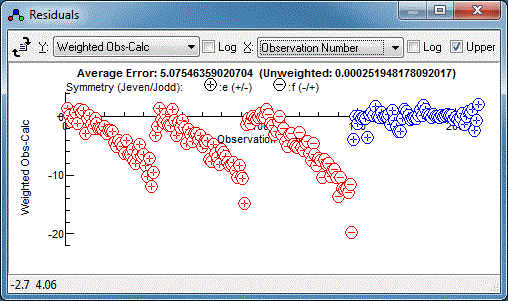
The Colour directives in the control file govern the colour of
the points in the residuals window, and this makes it very clear
that the relative estimated errors of the two data sets need
adjustment:
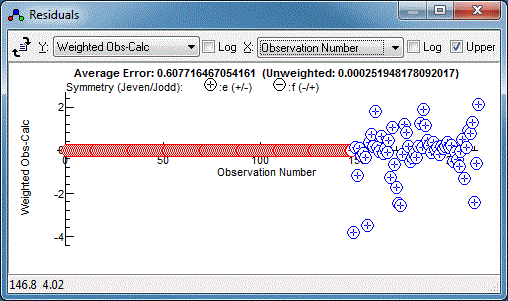
The microwave data has weighted residuals,
(Observed-Calculated)/Estimated Error, in the range of -3 to +3,
which is as expected if the estimated errors correspond to one
standard deviation, and indeed the .cat file has an individual
uncertainty assigned to each line. The infra-red data has a much
smaller range of residuals, suggesting estimated error is much
too large, and indeed the default of 1 that we used above is
much larger than the resolution of 0.001cm-1. (Note
that only the relative magnitudes of the estimated errors are
important in fitting, so the default of one is normally adequate
if the data is all from the same source.) We could edit the
estimated errors in N2OIRv1.obs but it is easier to
add an override in the control file, as in:
Colour Red
ScaleStdDev 0.001
include N2OIRv1.obs
ScaleStdDev
Colour Blue
include c044004edit.cat
The
ScaleStdDev
directive scales all subsequent estimated errors by the value
given, or 1 if no value given. In fact just scaling by the
linewidth still looks like too large an error:
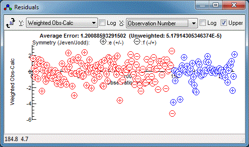
and a better guide is the average error in the infra-red fits,
5×10
-5. Using
ScaleStdDev 5e-5 gives:
The relative errors now look good, but there is clearly a
systematic error in the infra-red data. We can now do a combined
fit, floating everything we have floated before -
B,
D,
H and
L in the ground state, and the Origin,
B,
D,
q and
qD in the
excited state. A few fitting cycles gives:
suggesting a good overall fit. The files at this stage are
N2Ostage5.pgo and
N2Ocombined.obs.
7. More Advanced Fitting - Hot Bands
If you look carefully at the infra-red spectrum you can see two
additional weak Q branches in the spectrum, at 579.36 cm-1
and 588.98 cm-1. (The expand vertical scale button,  , is helpful in seeing the latter.) These are due
to hot bands, i.e. transitions where the lower state is a
vibrationally excited state, and in fact for these two branches
the lower state is actually the upper state of the infra-red
transition we have been working on so far. We expect P and R
branches associated with these Q branches to be present also,
but are going to be rather difficult to spot.
The v2=2 state of N2O will actually have
two components with bending quantum number l = 0 and 2
corresponding to Σ+ and Δ symmetry
respectively. To set up the data file to include these perform
the following steps in the constants window; we will start by
just adding a single state.
- Duplicate the upper (v2=1) state of the infra-red
transition by right clicking on "Excited" and
selecting "Copy With Linked Items" then right click
again and select "Paste".
- Some renaming is called for - the names are arbitrary, but
to reduce confusion right click on "Copy of Excited",
select "Rename" and enter "Second". Right click on "v=1"
below Second, select "Rename" and enter "v=2".
- This has copied the constants from v=1 to v=2 which is a
reasonable starting point for B but not the origin,
which will be about twice that for v=1. Try 1176 for this -
click on v=2 and enter this at Origin.
- Pressing the simulate button and then "All" will
show that the 2-0 overtone band is now visible in the
spectrum. This is not the required hot band, which we fix by
right clicking on <Second|mu|Ground>,
selecting "Rename" and changing "Ground" to
"Excited" in the resulting dialogue box.
- This will not (yet) produce any transitions in the
simulation. To make PGOPHER consider a manifold
(such as Ground or Excited here) as an
initial state in a transition the Initial flag must
be set. Click on "Excited" and change Initial
from False to True.
- There should now be some hot bands in the simulation, but
they are likely to be difficult to see as they are so weak. As
a quick fix, set the vibrational temperature, Tvib, to 3000 K.
(Click on the Simulation object in the constants
window for this.) This allows a different effective
temperature for the distribution over rotational and
vibrational energy levels, which you may need to simulate
spectra in some circumstances.
- To distinguish spectra from multiple sources colour coding
can help. Click on v=2 and change Colour
to Navy. Clicking on the "Individual Spectra"
button,
 , will then show the hot bands in
blue. You will need to turn off the display of the overall
spectrum with the "Show Sum" button,
  . Also
try cycling through the various plot styles with the "Next
Plot Style" button,
  .
.
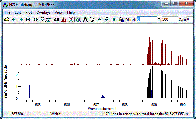
Your plot should now look something like this (the vibrational
temperature,
Tvib has
been reset to the default (-1) for this, implying the rotational
and vibrational temperatures are the same).

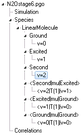
The data file at this stage is available as
N2Ostage6.pgo. The object tree
at this stage looks like:
Note there are several possible transition moments that could be
added to this picture, including
<v=1|T(1)|v=1>
under a
<Excited|mu|Excited> transition moments
object (which would give microwave transitions within v
2=1)
and
<v=2|T(1)|v=0> under a
<Second|mu|Ground>
object which, as we saw above, would simulate an overtone
transition.
To fit the Q branch at 579.36 cm-1:
- Adjust the v=2 Origin so the Q
branch hot band is in about the right place.
- The state type will not be right - try both Σ+ and
Δ for v=2. For the Δ state both q and
qD should be set to 0, as l doubling
is typically too small to be observed. (To avoid confusion
they should also be cleared for the Σ state, but only
because they are ignored for a Σ state.) This is a good
application for the mouse adjust function (F3) as only the
upper state constants (v=2) need adjusting. Good
values for the increments are 0.001 for the Origin
and 1e-5 for B. In addition the way lines merge is
important for the appearance of the spectrum here, so a width
should be added to the simulated spectrum. Try setting the
Gaussian width of the spectrum to 0.001 in the Gau
box at the top of the main window.
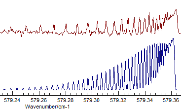
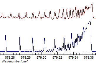
- The difference between Σ+ and Δ is fairly subtle
- the band selected is actually Σ+, and visually
the difference is that the transition to the Δ has two
branches, corresponding to the two different parities. Compare
(Σ+, Origin=1168.1305, B=.41992
available as N2Ostage7.pgo):

with (Δ, Origin=1168.1305, B=.41915):

Even given the assignment of the state symmetry, the assignment of
individual lines is awkward as the numbering of the of the peaks
is not easy to establish. This is made more difficult in this
case, as the centrifugal distortion constant,
D, is
important in determining the appearance of the spectrum, and also
the Q branch only nature of the spectrum means that common
differences are not available. A possible approach is to assign
the band head as the lowest
J transition (Q(1) in this
case), and then try a few different assignments. The
possible assignments will only differ in
J, and this is
easiest to change if the line list is in a text file. Try the
following:
- Bring up the line list window ("View", "LineList") and use
"Clear" to empty it. (The assignments currently in this window
have been saved above.)
- Assign as many lines as possible, floating the upper state
Origin, B and D to help this. It should be
possible to assign 20 or so lines with relative J
values correct even if you are not sure as to the absolute
numbering, so the band head won't necessarily look right
- Save the assignments in Branch format to a text file. (In
the line list window use "More", "Save To File", "In Branch
Format..." and save it to N2OIRv2SigmaBr.obs).
- This file requires a little editing before it can be used
for fitting; the upper and lower states must now be specified
as the edits above means there is now a choice. Edit the file
so it starts with:
UpperManifold Second
UpperState v=2
LowerManifold Excited
LowerState v=1
    Q(7)  579.3595            1 5.8582  : N2O_0.001....dpt - N2Onu2.ovr
    Q(8)  579.358             1 6.4287  : N2O_0.001....dpt - N2Onu2.ovr
    Q(9)  579.35695           1 6.9292  : N2O_0.001....dpt - N2Onu2.ovr
- In the branch format it is easy to slide all the assignments
along by one - simply change Q(7) to Q(8), Q(8) to Q(9) and so
on. Alternatively the BranchExpr
format format can be used by editing the file to look as
follows:
UpperManifold Second
UpperState v=2
LowerManifold Excited
LowerState v=1
BranchExpr Q(J)
  7 579.3595            1 5.8582  : N2O_0.001....dpt - N2Onu2.ovr
  8 579.358             1 6.4287  : N2O_0.001....dpt - N2Onu2.ovr
  9 579.35695           1 6.9292  : N2O_0.001....dpt - N2Onu2.ovr
(Versions of PGOPHER after 9.0.116 can also save directly to
this format from the line list window). To offset the
assignment replace BranchExpr Q(J) with BranchExpr
Q(J-1) or BranchExpr Q(J+1).
- Using either of the methods above try a few different
assignments, and look at the overall quality of the fit, and
how well the band head is reproduced. An offset of 2 from the
assignments given above gives the best fit to the band head:

8. Band Contour Fits
The spectrum above shows only partially resolved rotational
structure, and it may be worth trying a contour fit in these
circumstances. This fits directly to the observed spectrum,
rather than to line positions. While it sounds easier (in that
assignments are not required) a good starting point is required
as peaks must typically be within half a linewidth of their true
positions for the fit to succeed. For a spectrum like the one
used here contour fits only make sense as a follow up to a
standard line position fit. See Contour
Fitting for a full description.
For the current spectrum we use a slice of the original
spectrum at full resolution without averaging; this is available
at N2Onu2Sigmaonly.ovr.
(Fitting to the entire spectrum would not make sense.) Try the
following steps:
- In the overlays window
(View, Overlays), click on the topmost item and ensure that "IntensityUnits" are
set to "Normalized"
in both objects.
- In the constants window
(View, Constants) and click on "Fix", "Fix All
Parameters" and select "Mixture" to
ensure that no molecular constants are floated to start with.
- The first parameters to be floated must be the scale and
baseline of the overlayed spectrum. In the overlays window (View, Overlays),
float Scale and Baseline (click in the
float column so it reads “yes”).
- In the log window (View, Log)
choose "Contour"
as the fit type in the top left. On pressing the "Fit" button the main
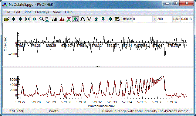
window will change to show two plots. The upper plot shows the
residual (the difference between the experimental spectrum and
the simulation) is shown in the main window (see below for an
example) and the lower plot the experimental and observed
spectra simultaneously. After a few cycles it should look
like:

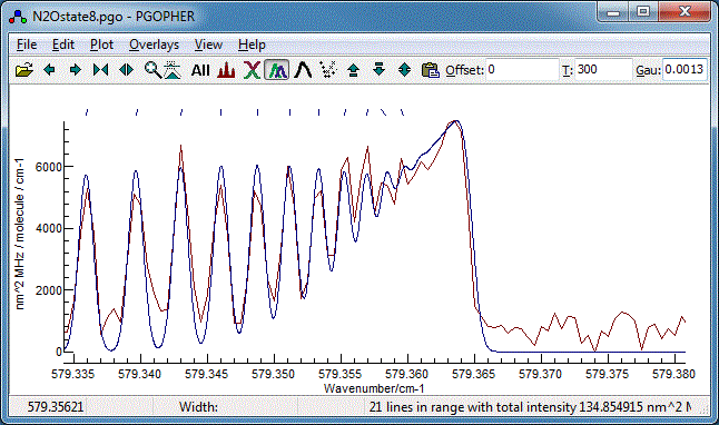
- This is actually quite good already, but try floating the
linewidth (Gaussian under the Simulation
object in the constants window), and Origin, B and D
for the upper state. You will find that the fit requires some
help to converge - the "Undo Fit" button,
 , is
essential here. A specific problem here is that the default
increments used for calculating derivatives for the least
squares fit are too large. This is a fairly common problem,
which is why the constants window allows setting an increment
for each parameter. Derivatives are calculated by repeating
the simulation with the parameter displaced by the increment,
and taking the difference from the initial simulation. Try
floating one extra parameter at a time, and if the fit
diverges use undo fit to step backwards to sensible values and
then experiment with the increment for the parameter. (Try
1e-8 for the Origin and 1e-13 for B). In this case a minor
improvement in the simulation is possible:

The final file is available as
N2Ostage9.pgo.
The overlay values used were Baseline=
0.02664,
Scale=91699.
9. Adding Custom Parameters - The Other Hot Band
The Δ - Π hot band at 588.98 cm
-1 is left as
mainly as an exercise for the reader, but some tips are in order:
- There are two different branches (corresponding to e and f
parities, showing as Qe(J) and Qf(J)) - turn on
the Fortrat plot to see this. There is significant overlap
between the two, so right clicking will often select more than
one transition. If this occurs, consider deleting one or more
of the lines before measurement. For initial fitting at low J
the f transitions are stronger, so try fitting the f
transitions only to start with.
- There are several possible ways to do this; in fact I picked
out a few f transitions and used the BranchExpr technique
described above to shift the assignment. To add more
transitions I then used the line list window as follows:
- Clear the line list window.
- Assign a few lines (Right click on the simulation, right
click and drag on the experimental spectrum.)
- Add to the line list file by pressing "All", "More",
"Copy Branch Table" in the line list window and using
paste in the editor with the line list file open.
- Fit with the new data, and then repeat from step 1.
The final line list file, N2OIRv2DeltaBrEx.obs
then contains a mixture of formats for the observations.
- Despite the earlier comment about l doubling being
typically too small to see for Δ state the resolution
here is sufficiently high to observe it, so q must be
floated for the Δ state.
- Even more unusually the centrifugal distortion of q
is also determined. This is not included in the standard
PGOPHER terms, but illustrates nicely how perturbations can be
used to add non-standard terms in a general way. See Λ Doubling and perturbation
objects for more details.
The final file is available at
N2Ostage10.pgo
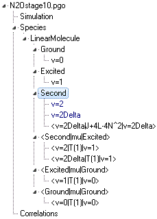
includes this perturbation. The object tree looks like:
The two v
2=2 states, v=2 (the Σ+ state) and
v=2Delta
(the Δ state), have been put in the same manifold (
Second).
These states, which are close together in energy, are a typical
case where one state might perturb the other so putting then in
the same manifold makes sense. This would allow the addition of a
Perturbation object to the manifold
to model the interaction. No interactions are observed here, so
the two states could equally be put in separate manifolds.
Left as an exercise for the reader is adding P and R branch
transitions from the hot bands to the observed line list - there
are some visible.
10. Using HITRAN data
Line lists from the HITRAN database
(or line listings with the same format) are understood by PGOPHER
and can be used in several different ways. At its simplest, the
line positions and intensities can be overlaid as an
"experimental" spectrum, but the files can also be used as input
to line position or intensity fits (PGOPHER can use the
quantum numbers in the file directly) or imported as an external
source allowing more general application of many of the features
of PGOPHER, such as energy level plots, in addition to
standard simulations. See Using HITRAN
files for further details.
The file N2OHITRAN2012v2edit.par
was obtained from HITRAN, in this case by using HITRAN on the
web at http://hitran.iao.ru/.
Browse to “Molecules”, select Nitrous Oxide
(molecule 4), select the ν2 band (0110 - 0000), hit
“Simulate Spectrum” and then select “Numerical
Representation” and save the resulting text. To trigger
PGOPHER’s processing of HITRAN files the extension
should be .par.
Alternatively, use the newer HITRAN online at http://hitran.org/. Select
“Data Access”, “Line-by-Line”,
“N2O”. In the “Select isotopologues”
page select 14N16O only. The frequency
ranges can be left at the default, but for the current exercise
“Select vibrational bands” is required. This option
is only available if you are logged in to the site, and
“Select by band” is turned on in your profile. In
this case select “Upper state” = 0 11 0
(1), “Lower state” = 0 00 0 (1) and make
sure the output format is selected as “.par (160
chars)”. Use the link to download the generated .par file.
This .par file can be used as an overlay - drag and drop the
the .par file onto the PGOPHER window of use "File",
“Load Overlay...”. The .par files have absolute
intensities, in units of cm2 cm-1 Molecule-1
at 296 K. To force the experimental overlay to use these units,
make sure the intensity units in the Overlays window ("View",
"Overlays") are set to cm2WavenumberperMolecule at
both the top level and the N2OHITRAN2012v2edit.par
object. To make PGOPHER use the same units, set the
same intensity units in the Simulation object in the constants
window.For the simulated intensities to be correct the
transition dipole must be set correctly; this is the Strength
parameter of <v=0|T(I)|v=0> in the constants
window. Manual adjustment suggests a value of 0.04 D is
required.
The .par file can also be used as a line list for fitting, in
the same way as the .cat files described above. If you try that
for the supplied files position fits suggests a systematic error
of 0.0002 cm-1 at low J (about 1/3 of the
linewidth, probably the result of a small calibration offset)
increasing to higher J (suggesting HITRAN is derived
from a larger range of J than here). You will also see a
systematic difference in intensities, suggesting a Custom Transition Moment
is required.
HITRAN files can also be imported into PGOPHER using
“File, Import, HITRAN File....” The resulting file
will produce simulations in the normal way, allowing the
temperature and linewidth to be adjusted and right clicking on
any transition will give the underlying quantum numbers. Note
however, that two extra steps will normally be required to
produce complete results:
- If more than one isotopologue is present in the file the
abundances for each will need to be entered manually.
Importing the complete HITRAN file for N2O
will produce several HITRANMolecule objects named
41, 42, 43, ... corresponding to the HITRAN numbers. 41
corresponds to the main isotopologue, and the others can be
deleted or the Abundance set to the correct value in
the Molecule object. (Strictly the abundance should be set to
0.990333 rather than the default of 1)
- By default, the partition function is calculated by summing
over the energy levels deduced from .par file. This can give a
good starting point, but may not be correct. This is because
relevant levels may have been excluded from the HITRAN line
list and also the process of deducing the effective energy
level pattern from the line list is not foolproof. (Any error
this introduces will not affect relative intensities at a
given temperature.) To correct this, specify the partition
function as a table of values using an Interpolated Partition
Function. To add this, right click on the HITRANMolecule
object and select "Add New...", "Interpolated Partition
Function" and then right click on the Interpolated
Partition Function object, select "Load..." and then
select a file with the required values. HITRAN online makes the
requiered file available under "Documentation",
"Isotopologues". Look for the link to q21.txt.
An exercise for the reader is to use this import process to verify
the assignments above.
![]() )
button. The other key controls are:
)
button. The other key controls are:
![]() ) button to update the simulation and use
the zoom to selected (
) button to update the simulation and use
the zoom to selected (![]() ) button to just display the band of
interest.
) button to just display the band of
interest.


![]() ). The
resulting plot has the same horizontal axis as the main plot,
but J as the vertical axis. This allows individual
branches to be picked out. A symbol is plotted for each
transition, and the size of the symbol proportional to the
intensity:
). The
resulting plot has the same horizontal axis as the main plot,
but J as the vertical axis. This allows individual
branches to be picked out. A symbol is plotted for each
transition, and the size of the symbol proportional to the
intensity:


![]() , is helpful in seeing the latter.) These are due
to hot bands, i.e. transitions where the lower state is a
vibrationally excited state, and in fact for these two branches
the lower state is actually the upper state of the infra-red
transition we have been working on so far. We expect P and R
branches associated with these Q branches to be present also,
but are going to be rather difficult to spot.
, is helpful in seeing the latter.) These are due
to hot bands, i.e. transitions where the lower state is a
vibrationally excited state, and in fact for these two branches
the lower state is actually the upper state of the infra-red
transition we have been working on so far. We expect P and R
branches associated with these Q branches to be present also,
but are going to be rather difficult to spot.