Energy Level Plot Window
This window can be used to display a wide variety of energy level
plots. The plot below is a typical linear molecule plot, showing
the rotational levels of the ground X 3Σ -state
of SO. Plotted as a function of J,
in shows the F1 F2 and F3
components as a function of J.
Note that BJ(J+1) has been subtracted from
the vertical scale, so that the deviations from the simple BJ(J+1) pattern are clear. The actions of the
various controls are listed below.
- The status bar at the bottom will show
the co-ordinates of the mouse at a minimum, and will also
normally show information about calculated and observed points
if over a point.
- To print the plot right click on the plot and
select "Copy to clipboard" and then paste it into a
suitable application. For Microsoft word, and many other
applications it is important to use "paste special" rather than
a simple paste (otherwise the numbers producing the plot will be
pasted, rather than the plot itself).

  |
Select which states to plot. |
 |
Write the plotted energy levels to the Log window |
 |
Open another level Window |
Plot Type
 |
The options in this group control the overall appearance
of the plot.
|

|
Plot against external field, rather than quantum number.
See Electric or Magnetic Field
Plots for more details.
|

|
Select to plot absolute symmetry, rather than
J adjusted symmetry.
|
 |
Plot a symbol for each level. The key to the symbols will
normally be shown at the top of the plot, and different
symbols indicate different symmetries.
|
 |
Join associated levels with lines. The levels joined are
controlled by the three options below.
|
 |
Plot both points and lines.
|
 |
Choose between starting join process from the highest
energy or lowest energy point |
 |
Try to join points with related values of quantum numbers |
 |
Try to join points arising from same state |
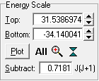
Energy Scale
 |
The options in this group control the vertical scale of
the plot
|
  |
Maximum energy in plot |
  |
Minimum energy in plot |
 |
Refresh Plot (only needed if
AutoReplot turned off in mixture) |
 |
Adjust plot range to include all levels |
 |
Zoom to selected vertical range |
 |
Compress vertical scale |
   |
Subtract number × J(J+1) from all energies
plotted |
Level Selection
 |
This group allows levels to be selected by symmetry or
some other quantum numbers. The picture is for a linear
molecule; alternate quantum numbers are selected for other
molecule types.
|
  |
Select (or not) symmetry to plot |

|
Limit J range plotted to Jmax
for manifold.
|
  |
Select Ω (linear molecules), Ka (asymmetric tops) |K| (symmetric tops) or
v1 (Vibrating molecule).
|
  |
Select Fn (linear
molecules), Kc
(asymmetric tops) or Kl
(symmetric tops).
|
x Axis
 |
For normal plots, this controls the x axis.
|
  |
Select quantum number for x axis |
  |
Minimum J to include in plot |
  |
Maximum J to include in plot |
Observed Level Overlay
 It is possible to compare calculated
and observed energy levels, with the "observed" energy levels
calculated by combining the measured line positions with the
calculated energy levels for the other state. This requires an
experimental line list (a .lin file), made as described in line position fitting. To include
experimental information:
- Make sure the line list file is set in the Log window.
- Select
 to plot upper state energy
levels or
  to plot lower state energy levels.
- Press
 to display the
observed energy levels.
- The display is normally clearer if
 is selected for the calculated energy levels.
- If the mouse is over an experimental point it's source is
displayed in the status bar; right click offers the following
options:
- Edit Point: Open point under cursor in editor if possible.
- Show Line: Centre main plot on transition
 |
Plot Upper State Observed
Levels: Eobs = Elower +
νobs |
 |
Plot Lower State Observed Levels: Eobs
= Eupper - νobs |
 |
Join observed point to calculated point |
 |
(Re)load observations |
  |
When plotting observed energy levels, scale the distance
from the calculated position by this. If a negative value is
given, then the plotted point is Ecalc +
(Eobs-Ecalc)/σ,
where σ is the estimated error of the observation. If
Exclude Perturbations is
set, then perturbations are excluded from calculating Ecalc,
but not from the Elower or Eupper
value used in calculating Eobs. |
Calculation Adjustment
 |
This group allows the selected items to be excluded from
calculations
|
 |
Exclude perturbations in plotted levels |
  |
Set how many nuclear and electron spins to exclude from
the calculation |
Line Labels
Where to place labels on calculated lines. Possible choices are:
 |
- None
- LeftOut: At left edge of plot, right justified
- LeftIn: At left edge of plot, left justified
- RightIn: At right edge of plot, right justified
- RightOut: At right edge of plot, left justified
- Start: At start of the line
- End: At the end of the line
|


 It is possible to compare calculated
and observed energy levels, with the "observed" energy levels
calculated by combining the measured line positions with the
calculated energy levels for the other state. This requires an
experimental line list (a .lin file), made as described in line position fitting. To include
experimental information:
 to plot upper state energy
levels or
  to plot lower state energy levels.
 to display the
observed energy levels.
 is selected for the calculated energy levels.


