Contour Fitting
Contour fitting allows fitting the overall shape of an
experimental spectrum to a simulation, and is useful for low resolution
spectra in which the rotational structure is not fully resolved. Note
that the results from this sort of fit are typically less reliable than
for a line position fit, and a line
position fit is to be preferred if at all possible.
- To start a contour fit, Overlay the
experimental spectrum over the PGOPHER simulation. The initial
match
must be quite good for a contour fit to work - a contour fit will
typically not move a peak more than the peak width, for example.
- It is easier to work if the intensity units of both the overall
overlay, and the specific overlay(s) to be floated are set to "Normalised", rather than
arbitrary. Go to the overlays
window (View, Overlays), click on the topmost item and ensure that "IntensityUnits" are set to "Normalized". Click on the
specific overlay and check the same setting. After doing this the "Baseline" and "Scale" will need to be adjusted
for a reasonable match with the simulated spectra as the vertical
autoscaling is now turned off.
- Open the constants window
(View, Constants) and click on “Fix all” to ensure that no molecular
constants are floated to start with.
- The first parameters to be floated must be the scale and
baseline of
the overlayed spectrum. Go to the overlays
window (View, Overlays), select the overlay required (probably the
first one unless you have more than one experimental spectrum overlaid)
and float these two parameters (double click in the float column so it
reads “yes”).
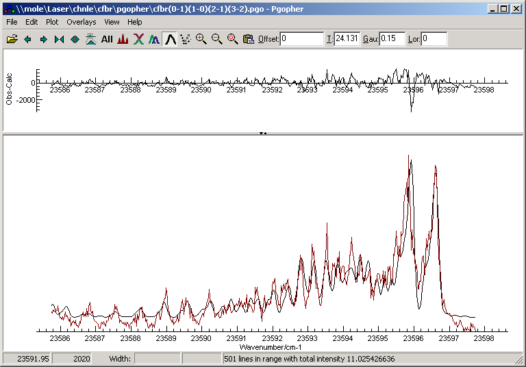
- “View”, “Fit log”, and choose “Contour Fit”. A separate plot
showing the obs-calc (difference between the experimental spectrum and
the simulation) is shown in the main window (see below for an example),
along with the simulation. The “Log” window now shows new values for
the floated
parameters and
their errors, the average error, and a correlation matrix. The error
will typically be very large at this point
- Press “Contour Fit” repeatedly, until the average error is as
low as possible, and a simulation that roughly matches the experimental
spectrum is shown. If you have problems you may have to fix some of the
parameters and try manually changing them.
- To further improve the fit, start floating
molecular parameters. Floating many parameters simultaneously will
often cause the fit to make wild changes in some of the parameters
unless the fit is very good. For best results float additional
parameters one or two at a time, starting with the most important. The
Undo Fit button allows you go back to previous fits, if you find you
have gone too far from a reasonable fit. For example, the excited state
origin might be the first
molecular constant to float (“View”, “Constants”, and double click on
the “no” next to the constant to change it to yes.). Again, press
“Contour fit” repeatedly until the error reaches a minimum, and
converges.
- Other parameters to consider are A or B
rotational constants, the linewidth and rotational temperature.
Eventually, the simulation should closely resemble the experimental
spectrum, and the obs-calc will be much smaller.

