| |
<Prev Next> |

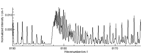
This example is based on A. S-C. Cheung, W. Zyrnicki and A. J.
Merer, J. Molec. Spectrosc. 104 315 (1984), and shows an
example of a spectrum involving states with high
multiplicity, and also demonstrates two alternative approaches
to dealing with molecular parameters that are not presented in
quite the same way as PGOPHER requires them. Four
slightly different data files are given below. The difference
between them is not really significant on the scale of the
precision of the original data, but CrOAdjusted.pgo is the
recommended one to use.
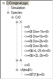
CrOOriginal.pgo. This
gives the data in a form that is closest to the form presented
in the paper, which requires special consideration as follows:
 The origins of the individual components of the
ground X5Π state are specified individually, rather
than in several spin orbit coupling constants. This effect can
be achieved in PGOPHER using perturbations, in this
case homogeneous contributions with OmegaSelect set.
For example <v=0|Om=3|v=0> shifts the Ω = 3 component
(only) by the amount of the perturbation Value. For
correct assignment of the quantum numbers PGOPHER requires an
approximately correct value for the spin-orbit coupling
constant, A, so not all the components can be positioned in
this way. For the file given here, the Ω = 0 and 1 components
are fixed by setting the state Origin and A
values, and perturbations are used to position the other
spin-orbit components. In this case it is possible to derive
the values by comparing the matrix elements used in PGOPHER
and the paper, though in general it can be simpler to simply
re-fit data from the literature.
The origins of the individual components of the
ground X5Π state are specified individually, rather
than in several spin orbit coupling constants. This effect can
be achieved in PGOPHER using perturbations, in this
case homogeneous contributions with OmegaSelect set.
For example <v=0|Om=3|v=0> shifts the Ω = 3 component
(only) by the amount of the perturbation Value. For
correct assignment of the quantum numbers PGOPHER requires an
approximately correct value for the spin-orbit coupling
constant, A, so not all the components can be positioned in
this way. For the file given here, the Ω = 0 and 1 components
are fixed by setting the state Origin and A
values, and perturbations are used to position the other
spin-orbit components. In this case it is possible to derive
the values by comparing the matrix elements used in PGOPHER
and the paper, though in general it can be simpler to simply
re-fit data from the literature.As an example of how this can be done, consider the diagonal Ω = 0 matrix elements given in the paper for the X5Π state (Table I):
T0
+ (B-AD-2LambdaD+/-3*oD)*(J*(J+1)+5)
- D*(J*J*(J+1)*(J+1)+20*J*(J+1)+25)
+/-3*(o+p+q)
PGOPHER gives the following for the same matrix elements (right click on X and select matrix elements):
<J,Lambda=1,Omega=0 + |H| + J,Lambda=1,Omega=0> =
+  Origin
+  B*(J*(J+1)+5)
+  -A
+  + 3*o
+  -6*gamma
+  D*(-J*(J*(J*(J+2)+21)+20)-25)
+  (AD+2*LambdaD)*(-J*(J+1)-5)
+  +3*oD*(J*(J+1)+5)
A little algebra will show that these two expressions are identical apart from o and oD (discussed below) and the J independent terms. Equating these shows that TO = Origin-A-6*gamma. Repeating the process with Ω = 1 shows that T1 = Origin-6*gamma. The difference between these, T1 - T0 = A, so given that the paper fixes T0 = 0 it follows that A can be set to T1. The paper has chosen to take the energy zero for the state at Ω = 0, while PGOPHER will take it at Σ = 0 component (Ω = 1 here). To align the two scales, set the PGOPHER Origin = A+6*gamma. Repeating the process for the other Ω components gives the following set of equations:
T(-1) = Origin-2*A-4*gamma+<v=0|Om=-1|v=0>
T2 = Origin+A-4*gamma+<v=0|Om=2|v=0>
T3 = Origin+2*A+<v=0|Om=3|v=0>
Note that the homogeneous perturbations such as <v=0|Om=3|v=0> have been added here, and each of these is essentially indicating how far the component has been shifted from the equal spacing predicted from the simple spin orbit energy formula AΛΣ. The required value for each component can be worked out by rearranging the above giving, for example, <v=0|Om=2|v=0> = T2-T0 - (2A+2*gamma).
FrequencyOffset -54.43912
NQN 2
 - - 1 F1f 0.0002
 - - 2 F1f 2.025
 - - 3 F1f 5.0621
 - - 4 F1f 9.1117
 - - 14 F1f 105.3185
 - - 15 F1f 120.5138

 - - 0 F2f 57.1558
 - - 1 F2f 58.1881

 - - 0 F2e 56.9666
 - - 1 F2e 58.0008
 - - 2 F2e 60.0692
 - - 3 F2e 63.1718
Only a few entries have been included. Notes on producing this:
Given the settings above, table VIII can be reproduced exactly
if minor adjustments by fitting are made to the Origin, B, o,
gamma and the perturbations. The adjustments are mainly because
the constants have not been quoted to sufficient precision to
reproduce the calculated values.
The transitions given in the appendix can be similarly
converted into a form that PGOPHER can read using the BranchTable
format:
BranchTable sR54 rQ54  qP54    pQ34      oQ24     oP34     nP24
7  8021.3   8011.337    -        -        -        -        -
8  8023.748 8012.779 8002.799    -     7988.457    -        -
9  8026.122 8014.157 8003.182    -     7986.855    -        -
10 8028.406 8015.457 8003.513    -        -        -     7976.194
11 8030.687 8016.698 8003.742    -     7983.441    -     7973.451
12 8032.814 8017.876 8003.909    -     7981.63     -     7970.649
13 8034.913 8018.965 8004.007    -     7979.758    -     7967.778
14 8036.943 8020.003 8004.04  7992.332 7977.818    -     7964.822
15 8038.898 8020.967 8004.007 7991.327 7975.811 7976.352 7961.852
16 8040.787 8021.867 8003.909 7990.252 7973.74  7974.309 7958.792
Again, only a few sample lines are shown. The agreement with
the observed lines is good, but can be slightly improved
(average error dropping from 0.011 to 0.0086 cm-1) by
fitting the upper state Origin, B and LambdaD. The changes are
minor, with the exception of LambdaD which changes from 4.6e-6
to 1.6e-6. This may reflect a misprint in the original paper, or
possibly a more thorough treatment of blended transitions in the
original fit.
CrO.pgo is set up using the
standard constants available in PGOPHER, derived as follows: