Worked Example - The Schumann-Runge Bands of O2
The key parameters required for a
simulation of a linear molecule spectrum are summarized in
Making a Linear Molecule Data File. The
steps below show how to do this for part of the Schumann-Runge
Bands of O
2, which are responsible for atmospheric
absorption around 190nm.
The Constants
The molecular parameters are
required for any simulation; an excellent compilation of constants
for diatomic molecules can be found in the NIST Chemistry web book
at
http://webbook.nist.gov/chemistry/.
This database includes an electronic version of information in the
book K.P. Huber and G. Herzberg, "Constants of Diatomic
Molecules". A formula search on O
2 with "Constants of
diatomic molecules" selected yields many states; the
Schumann-Runge Bands arise from the B
3Σ
u-
- X
3Σ
g-. (The ν
00
value can be a helpful guide here as to which band to use.) An
abbreviated version of the table is presented below, with just the
B and X state entries.
| State |
Te |
ωe |
ωexe |
ωeye |
Be |
αe |
γe |
De |
βe |
re |
Trans. |
ν00 |
| B 3Σu- |
49793.28 |
709.31 a Z |
10.65 a |
-0.139 |
0.81902 a b |
0.01206 a |
-5.56E-4 |
4.55E-6 c |
|
1.60426 |
B ↔ X R |
49358.15 Z |
| X 3Σg- |
0 |
1580.193 Z |
11.981 d |
.04747 |
[1.4376766] e |
0.01593 f |
|
[4.839E-6] e |
|
1.20752 |
|
|
The footnotes contain the source of the information, and also some
additional constants that are often essential to obtaining a
reasonable simulation including the the spin orbit coupling
constant,
A (required if
the electron spin and orbital angular momentum are both non zero)
and and the spin-spin coupling constant, λ (required if the
electron spin is >= 1;
LambdaSS
in
PGOPHER). The
more important ones are referenced in the in the table above:
a) ω
eye
= -0.139, γ
e = -0.00055
6 from a low order
fit to v ≤ 4.
b)
The spin splitting
constants at low v are λ = 1.5, -γ ~ 0.04 cm
-1.
c) β =0.22E-6 for low v.
d) ω
eze
= -0.00127
3
e) Spin splitting constants λ
0
= +1.9847511, γ
0 = -0.00842536;
f)
B1
= 1.42192
Vibrational Dependence of The Constants
Much of this information is concerned with the variation of
constants with vibrational number, v. The numbers in the main
table are not suitable for direct entry into
PGOPHER, as they are
equilibrium values. For each vibronic transition, with a
particular v' and v" a separate set of constants is required. To
choose a specific case we will simulate the B
3Σ
u-
v' = 2 - X
3Σ
g- v" = 0 transition.
The band origin
E(v)
=
Te + ωe(v + ½) − ωexe(v + ½)2 + ωeye (v + ½)3 + ωeze (ν + ½)4
For B3Σu- v' = 2 this gives:
Origin = 49793.28 + 709.31(2 +
½) − 10.65(2 + ½)2 + -0.139 (2 +
½)3 = 51497.82 cm-1.
Note that ωeze is not given, though footnotes
not reproduced here indicate more information is available; G(v)
values or band origins are normally the values tabulated in the
primary literature.
For X3Σg- v" = 0 this gives :
Origin = 1580.193(0 +
½) − 11.981(v + ½)2 +
0.04747(0 + ½)3 + -0.001273(0 +
½)4 = 787.11 cm-1. Here ωeze is given.
The band origin for the transition is then 51497.82 - 787.11 =
50710.71 cm-1. Note that either the two separate origins
can be entered, or the ground state origin can be left at zero and
the difference entered for the excited state origin
The Rotational Constant
A similar process is required for the rotational constant; the
equation is similar:
Bv = Be − αe(v +
½) + γe(v +
½)2 + ...
For B3Σu- v' = 2 this gives:
B2 = 0.81902
− 0.01206(v + ½) + -5.56E-4(v +
½)2 = 0.785395 cm-1.
For X3Σg- v" = 0 the [] indicates
that the value is for v = 0 so no evaluation is necessary; a value
for v = 1 is given in the footnote and references to sources for
higher v are given in the full table.
The centrifugal distortion constants follow a similar equation:
Dv
= De − βe(v + ½) + ...
though this can be omitted for a rough simulation.
Other Constants
The spin-orbit (A) and
spin-spin (λ) constants are also often crucial to obtaining a
reasonable simulation; in this case the spin-orbit constants are
zero as both states are Σ, but the spin-spin constants are required
as S = 1. Both are only given in the footnotes:
For B3Σu-
v' = 2, λ = 1.5
For X3Σg- v" = 0, λ = +1.9847511
The spin-rotation constant, γ, is also given for these two states,
though this is normally less important.
Setting up the simulation
There is now enough information to produce a basic simulation in PGOPHER:
- Click on File,
New, Linear Molecule
- Select View, Constants
- Click on LinearMolecule. This sets the parameters common to
all states, and the ones that need to be changed from the
default values are:
- Symmetric = "True" (as the
molecule has a centre of symmetry)
- AsymWt = 0 (This is
the statistical weight of antisymmetric states, and the zero
reflects the fact that half the levels of O2 are
missing.
- Click on "v=0" and enter the information for X3Σg-
v = 0
- Lambda = Sigma-
- S = 1 (the electron spin)
- gerade = True (the default,
indicating g
symmetry)
- B = 1.4376766
- LambdaSS (λ) = 1.9847511
- Click on "v=1" and enter the information for B3Σu-
v = 2
- Lambda = Sigma-
- S = 1 (the electron spin)
- gerade = False (to indicate u symmetry)
- Origin = 50710.71
- B = 0.785395
- LambdaSS (λ) = 1.5
- To avoid confusion the "v=1" name should be changed; right
click on "v=1" and select rename to do this. The name does not
affect the calculation, but "v=2" would be the logical choice!
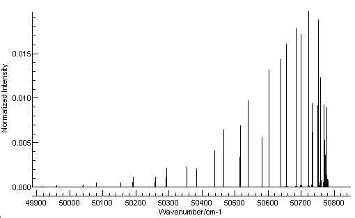
This should be enough to for a
basic simulation; press the simulate button (

) and then the all button (

) and you should see a simulation.
With a small adjustment of the plot range it should look like
this:
Checking and refining the simulation
It is important to check the simulation, not
only because it is easy to make mistakes in the steps above, but
also because there can be differences in the definitions of the
constants used. Checking against tabulated line positions or
published spectra is an effective check; note the
facility for overlaying pictures
(from a Journal for example) onto a simulation.
In this case a numerical spectra is available
from the Harvard-Smithsonian Center for Astrophysics website (
http://cfa-www.harvard.edu/),
specifically
the
CfA
Molecular
Data. For oxygen, measured cross sections are available;
follow the links
Measured
cross
sections: Schumann-Runge bands of all isotopes, 179 nm - 203 nm,
(2,0) band, 50050-50720 cm-1 . This gives a table
of numbers which can be directly copied into
PGOPHER; in your browser
use "select all", "copy" and then in
PGOPHER use "Overlays, Paste". The observed
spectrum will appear above the simulation.
Following the instructions above gives a
spectrum a reasonable simulation, and a good visual match can be
obtained with a Lorentzian linewidth of 0.65 cm
-1 (The
"Lor" box on the main window toolbar). The width does not take
effect in the simulation if the display is too compressed; zooming
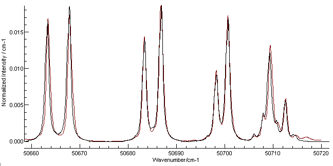
in to the portion around the band origin gives the following plot:
Here the red line is the Harvard data and the black is the
simulation. The most obvious discrepancy is on the right, and is
most likely a transition from another band. The line positions are
not absolutely perfect, but this could be improved by adding
D and γ to the simulation and
checking the literature for more accurate constants. The overall
experimental spectrum also shows additional lines at the other
end, probably from the (4-1) band. (An obvious exercise for the
reader is to check this using by following the procedure above for
this band.)
 ) and then the all button (
 ) and you should see a simulation.
With a small adjustment of the plot range it should look like
this:
