| |
<Prev Next> |
In this example we will go through the process of analysing the
spectrum shown below which is a fragment of the ultraviolet LIF
spectrum of C3. This will highlight some of the
considerations that go into assigning and simulating a spectrum.

This spectrum is available as C3AX.ovr. The near UV electronic spectrum of C3 is known to be dominated by an A1Πu - X1Σ+g transition, and a rotational constant of ~0.5cm-1 is typical for a molecule of this size. This gives us enough information to set up a basic data file, as summarized in Making a Linear Molecule Data File. Setting this up, with an origin of 27178 cm-1and a temperature of 30 K, remembering to set AsymWt = 0 as there are two equivalent spin zero nuclei gives the following simulation:
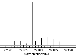
This shows a strong Q branch, which is clearly present in the
experimental spectrum at around 27178 cm-1and the
branch to the right looks as though it could be assigned - note
the small gap immediately to the right of the Q branch, which is
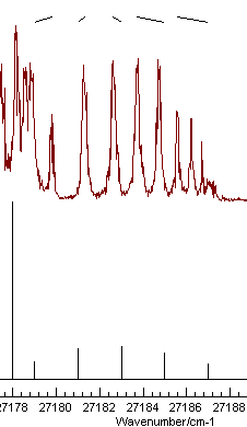
also visible in the spectrum. Using the Line
Position Fitting procedure to assign the first few members
of this branch, starting from the left gives the picture on the
left on pressing "Test":
 |
 |
| Good |
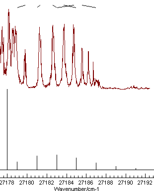
Mis-assignment |
Note the nice pattern of indicating marks at the top for the spectrum on the left, joining the positions of the observed and calculated line positions. The plot on the right shows a typical plot following a mis-assignment.
We can now try some fitting; it normally makes sense to start by fitting just a few parameters, so let's try the upper state origin and B:
5 Observations,  2 Parameters
Initial Average Error: 1.22114672883084
Predicted New Error:   0.34497794153667
Parameters:
  # Old                 New                 Std Dev   Change/Std Sens    Summary              Name
  1 27178               27178.5648453395    .2402865     2.3507  .017249 27178.56(24)         A v=1 Origin
  2 .5                  .474483017372344    .0048478    -5.2636  .000348 0.4745(48)           A v=1 B
These two parameters are well determined, and the plot shows a
much better fit:
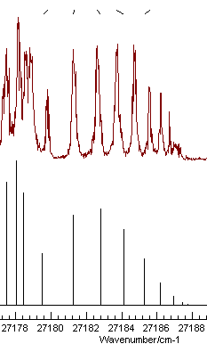
It also indicates one of the lines has been mis-assigned - the
rightmost one. Note that holding the mouse over the tick mark at
the top will show the source of the relevant observation, and
right clicking will take you to the line in the linelist window
for editing. Correcting the error and re-fitting gives an even
better fit. The obvious additional parameter to float is the lower
state B value, and the fit with these observations does
indeed work:
5 Observations,  3 Parameters
Initial Average Error: 0.0229832236953073
Predicted New Error:   0.0229832236953073
Parameters:
  # Old                 New                 Std Dev   Change/Std Sens    Summary              Name
  1 .431694643119403    .431694642718755    .00863921    0.0000  1.99e-5 0.43169(864)         X v=0 B
  2 27178.9571892846    27178.9571892862    .033426      0.0000  .000766 27178.957(33)        A v=1 Origin
  3 .409391071646742    .409391071313973    .00714522    0.0000  1.55e-5 0.40939(715)         A v=1 B

Correlation Matrix
       1       2       3
  1   1.000
  2  -0.878   1.000
  3   0.999  -0.894   1.000
While the values are physically reasonable, note the large correlation of 0.999 between parameters 1 and 3, the two rotational constants, which is also reflected in the estimated errors for these parameters being quoted to 3, rather than 2 figures. This implies that there is only just enough information in the supplied data to determine the three parameters, and the derived values should be looked at with some suspicion.
The correlation can be broken by adding more
lines, preferably from another branch. Looking at a wider range of
the spectrum indicates several possible extra assignments, though
there are clearly more lines in the experimental spectrum than the
simulation, indicative of an additional band being present:
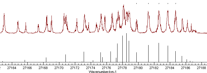
At this stage it is probably simplest to add
several assignments, and then look for any that don't look quite
right. Assigning 14 more lines that look about right leads to an
improved fit:
19 Observations,  3 Parameters
Initial Average Error: 0.0585913375363875
Predicted New Error:   0.0585913375363875
Parameters:
  # Old                 New                 Std Dev   Change/Std Sens    Summary              Name
  1 .429544716011829    .42954471601421     .00101655    0.0000  2.03e-5 0.4295(10)           X v=0 B
  2 27178.9692155569    27178.969215557     .02145922    0.0000  .001953 27178.969(21)        A v=1 Origin
  3 .408140469786951    .408140469789101    .00094343    0.0000  1.93e-5 0.40814(94)          A v=1 B

Correlation Matrix
       1       2       3
  1   1.000
  2   0.227   1.000
  3   0.976   0.058   1.000
Note how the correlation between the the rotational constants
(parameters 1 and 3) is no longer 0.999. At this stage the
residuals window (View, Residuals) is perhaps the best way of
looking for problems; compare the fit on the left with the one on
the right where one assignment has been shifted to the other peak
of a doublet (the pair at 27170.5 cm-1):
|
|
|
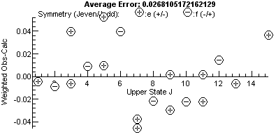
Note the plot on the right has a bigger vertical scale, and one
point, the mis-assigned peak, stands out. For a good fit, the
residual fit should look completely random, and a useful trick to
indicate issues is to try different horizontal scales. The plot
above are against upper state J, and the errors are
clearly bigger at higher J. This might be a cue to try
centrifugal distortion (D), though in this case note that
the f parity levels (minus signs in circles) are above the
axis and the e (+) levels are below the axis. This is a
classic symptom of lambda doubling, and allowing q in the
upper state to float gives a much improved fit, and the residual
plot now has no obvious trend:
19 Observations,  4 Parameters
Initial Average Error: 0.0301742415918127
Predicted New Error:   0.0301742415918126
Parameters:
  # Old                 New                 Std Dev   Change/Std Sens    Summary              Name
  1 .430438760425889    .43043876044772     .00053537    0.0000  7.85e-6 0.43044(54)          X v=0 B
  2 27178.9607318607    27178.9607318605    .01110167    0.0000  .000754 27178.961(11)        A v=1 Origin
  3 .409363044507011    .409363044540297    .0005115     0.0000  7.47e-6 0.40936(51)          A v=1 B
  4 -.00117830836843453 -.00117830840808154 .00016929    0.0000  1.49e-5 -1.18(17)e-3         A v=1 q

Correlation Matrix
       1       2       3       4
  1   1.000
  2   0.201   1.000
  3   0.972   0.025   1.000
  4  -0.209   0.095  -0.313   1.000
If you don't float the right parameters there are
various possible indications. If you float p (the other
commonly used lambda doubling parameter) instead of q
then PGOPHER clearly detects this is not determined:
19 Observations,  4 Parameters
Initial Average Error: 0.0620577920690341
Predicted New Error:   0.0620577920690341
**** 1 combinations of parameters not floated ****
Parameters:
  # Old                 New                 Std Dev   Change/Std Sens    Summary              Name
  1 .429658997291519    .429658997292251    .00107669    0.0000  1.61e-5 0.4297(11)           X v=0 B
  2 27178.9680780115    27178.9680780115    .02272882    0.0000  .001551 27178.968(23)        A v=1 Origin
  3 .408250076142484    .408250076143445    .00099924    0.0000  1.54e-5 0.40825(100)         A v=1 B
  4 0                   0                   NAN             NAN  INF     0 NAN                A v=1 p

Correlation Matrix
       1       2       3       4
  1   1.000
  2   0.227   1.000
  3   0.976   0.058   1.000
  4     Nan     Nan     Nan     Nan

Singular Value Decomposition
                        X v=0 B  A v=1 Origin       A v=1 B       A v=1 p
  1 606.33631228  -.68905037825 .005563083443 .724692092088 0
  2 42.9863049189 .724633451607 -.00956828901 .689068072586 0
  3 2.73019060661 .010767406567 .999938748098 .002561836805 0
  4 0             0             0             0             1
This case is particularly clear, in that the
singular value decomposition has indicated exactly which
parameter is not determined - the rows in the singular value
decomposition correspond to linear combinations of parameters,
the the lowest row indicates the combination that is least well
determined. In this case it is clearly p, and indeed
inspection of the Hamiltonian will indicate that p
requires non zero spin.
Floating D in either state gives a rather
better behaved fit, though the error bar is larger than the
parameter, indicating it should be fixed at zero:
4 -3.3058739831523e-7 -3.3059827872211e-7 3.3351e-6 0.0000 8.77e-8 -3(33)e-7 A v=1 D
Adjusting the temperature to 50 K and the
(Gaussian) linewidth to 0.25 cm-1 gives an excellent simulation
of most of the spectrum, though there is clearly an additional
band present:
