| |
<Prev Next> |
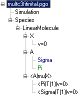
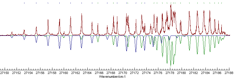
In this example we will show some of the considerations required when fitting multiple states simultaneously, particularly with regards to the putting the line lists together for fitting. We start where the single state fit in Fitting example - the A-X transition in C3 finished by adding another state. The experimental spectrum does not seem to show the presence of another Q branch, suggesting a Σ-Σ transition should be added. If we assume the lower state is the same for both transitions, then this can easily be generated by right clicking on the upper state, selecting "Copy with linked items" and then "Paste". (There is more than one way to structure the addition of a state - see the "Different Manifolds" section below for a discussion of this.) Manually adjusting the origin of the new state to 27166.8 gives a promising simulation:

To obtain this appearance the colour of the new state has been set to "Navy" and the Π state to "Green"; the file is saved as multc3fitinital.pgo. Now, while the simulation is quite good, note that the indicating marks at the top show a very poor fit, and fitting with the old line list will fail. Deleting the line list and starting again would work fine, but there are better ways to do this which we we will now explore.
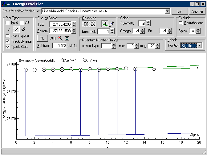
The origin of the problem introduced is best demonstrated by looking in the Energy Level Plot Window. Select "View, Levels", and for the best plot put the upper state rotational constant in the "Subtract" box, select the upper state manifold at "State/Manifold/Molecule", select line under "Plot Type" and both the buttons under "Observed". Pressing "All" should give a view like this:
If you have trouble setting this up, the settings are saved
in multc3fitinital.pgo.This
is a plot of energy against J, but with 0.408J(J+1)
subtracted from the energy, so simple states will give
horizontal lines. The two excited states are clearly visible
on this plot as the green and blue horizontal lines, and the
circles give the observed energy levels calculated from the
line list by adding the calculated lower state energy. The
vertical lines join the calculated to the observed energy
levels, and it is clear from this that about half some of the
assignments are to the wrong energy level. This is because the
line list constructed specifies states in terms of J,
symmetry (+ or -) and eigenvalue number, and we have just
added a state below the previous one, increasing the
eigenvalue number. There are various ways of dealing with this
and we work through several possibilities here, all of which
work for this case, but may not in more complicated cases.
The first possibility is to put the new state in a different manifold from the initial Π state. The original line list will then work, as the manifold is specified for each state. The disadvantage of this is that perturbations between states can't be simulated, and states close together in energy as these are may well interact. The required set in is shown in the right hand side below, with the original set up on the left:
 |
|
| Setup with two states (Sigma, Pi)
in a single excited state manifold (A) |
Setup with each state in
its own manifold (A for Pi,
Asigma for Sigma) |
Converting between the two is straightforward:
For the most flexible handling, the line list should be put
in a separate text file and edited with a separate text
editor, the The Slave Editor
included with PGOPHER or other text editor of your
choice. Use of a separate editor is more flexible than editing
in the line list window (undo/redo, search and replace), and
it is easy to combine separate sources of data into a combined
fit. To generate a file use "More, Save to File" in
the Line List Window, and then use
the Log Window to select the file
and fit.
The first option in fixing the line list is simply to change
the eigenvalue number that are wrong in the new simulation set
up. In the line list window this will be the #' column, and in
this case the values for the odd J levels need
increasing by 1. This change could be done manually, but a
further change may need making if a state is added or removed,
so we use the indexoffsets
directive. To use this we put the line list in a separate
file. Select "More, Save to File, In Standard Format"
in the Line List Window window and
choose a suitable filename, say APi.lin. Now go to
the Log Window, check than the file
you have just created is shown and press "Edit" to edit the
file. To add the required offsets add:
upperindexoffsets 1 0
at the start of the file and then save the changed file. (If
you use the the Slave Editor
included with PGOPHER this step is not necessary as
it a save is forced on each PGOPHER fit.) You can
check this is right by hitting the reload button in the Energy Level Plot Window and the
upper state should now show no long vertical lines, indicating
a correct assignment:

As an alternative the quantum numbers given in the comments
at the end of each line can also be used to work out the
eigenvalue number . In the Line List
Window this can be forced for an individual line by
clearing the eigenvalue number (#' and #") columns or in a
line list file by setting the eigenvalue number to 0. The
symmetry (S', S") can also be similarly left unset, though a
negative value, rather than 0 must be used in the line list
file to flag this. To force this for the entire file use:
upperindexoffsets search
to work out the eigenvalue numbers or
upperindexoffsets searchall
to work out both symmetry and eigenvalue number. Alternatively:
UpperState Pi
can be used to indicate that the eigenvalue numbers are to be
taken within the state. Any of these methods will work fine in
many cases, though where the quantum numbers are ambiguous,
typically in the presence of strong state mixing, the quantum
numbers assigned can change as the parameters change. In
fitting the quantum number assignments for any given state can
flip between successive fit cycles.
A few lines of the line list file are shown below; see Line List Input File Format for a
detailed explanation of each field.
LinearMolecule   A   1  1  1   X   0  0  1    27179.774 1 .03172      0 :     R(0) : A Pi  1 e - X v=0  0 e : LDS751.dr b - C3AX.ovr
LinearMolecule   A   3  1  1   X   2  0  1    27181.277 1 .05494      0 :     R(2) : A Pi  3 e - X v=0  2 e : LDS751.dr b - C3AX.ovr
LinearMolecule   A   5  1  1   X   4  0  1    27182.625 1  .0589      0 :     R(4) : A Pi  5 e - X v=0  4 e : LDS751.dr b - C3AX.ovr
...
Notes on this file:
UpperManifold A
1  1  1  0  0  1 27179.774 1
3  1  1  2  0  1 27181.277 1
5  1  1  4  0  1 27182.625 1
...
An alternative way of specifying transitions is to use
traditional branch notation, such as P(3), implying J'
= 2, J" = 3. Such a file can be generated from the Line List Window using "More,
Save to File, In Branch Format". The resulting file (in
APibranch.lin) looks like this:
For clarity, the intensity and comment fields have been removed. The "UpperState Pi" is required to identify which of the two possible upper vibronic states is required. defaultmolecule, uppermanifold, lowermanifold or lowerstate directives might also be required if there is more than one possibility for each.UpperState Pi
R(0) 27179.774 1
R(2) 27181.277 1
R(4) 27182.625 1
...
It is also possible to use the conventional quantum numbers
to specify the transitions. Such a file can be generated from
the Line List Window using "More,
Save to File, In Simple Format". The resulting file (in
APisimple.lin) looks like this:
For clarity, the intensity fields have been removed. The "UpperState Pi" is required to identify which of the two possible upper vibronic states is required. defaultmolecule, uppermanifold, lowermanifold or lowerstate directives might also be required if there is more than one possibility for each. The quantum numbers here are J' parity' J" parity"; see Simple Format for the possible formats of the quantum numbers. Note than NQN, the number of quantum numbers present for each state, must be specified.NQN 2
UpperState Pi
1 e 0 e 27179.774 1
3 e 2 e 27181.277 1
5 e 4 e 27182.625 1
...
NQN 2
 1 e  2 e    27164.765 1
 3 e  4 e    27163.026 1
...
To use this file with one of the previous Π state files set
up a separate file, say Aboth.lin,
with the following format:
Colour Green
Include APisimple.lin

Colour Navy
UpperState Sigma
Include ASigma.lin
The include statements simply read the contents of the given file. All the information could be put in one file, or split in any other way as convenient. The colour directives set the colour of the points in the Residuals Window and the indicating marks at the top of the main window. The final fit () gives an excellent overall simulation:
