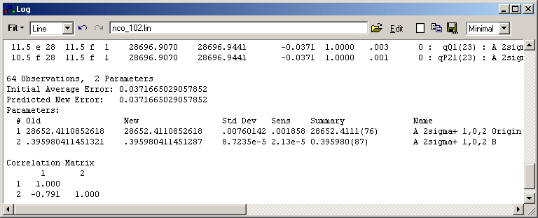
Observations
|
nobs = The number of
lines fitted or the number of experimental points for a
contour fit
|
Parameters
|
npar = The number of parameters
floated
|
Initial Average Error
|
This is [Σ[(obsi-calci)/wi]2/(nobs-npar)]½
with the calculated values, calci, obtained using
the parameters at their initial values. wi
are the estimated (relative) standard deviations of the
observations.
|
| Predicted New Error |
This is [Σ[(obsi-calci)/wi]2/(nobs-npar)]½
with the calculated values, calci, obtained from
the non-linear least squares fit. They are typically close
to the values that would be obtained from the new
parameters, but are only exact if the calculated values are
linear (or nearly linear) in the parameters. This is should
be the case near to convergence, but often not when starting
the fitting process. Fit again to find the true new error.
|
Old
|
The parameter value at the
start of the fit.
|
New
|
The parameter value after the
fit cycle.
|
Std Dev
|
The estimated standard
deviation of the parameter, based on the quality of the fit.
|
Change/Std
|
(New-Old)/Std Dev - the relative change in
the parameter.
|
Sens
|
Watson's sensitivity
parameter (J. K. G. Watson, J. Mol. Spectrosc. 66, 500 (1977)) for the
parameter. This is the change in the parameter that would
make the average error of the fit increase by a factor of
0.1/npar,
and provides a useful guide as to how many figures should be
quoted for the parameter to ensure that the calculation can
be reproduced. Where parameter correlation is high, this can
be many more figures than suggested by the standard
deviation of the parameter. See also R. J. Le Roy, J. Mol.
Spectrosc. 191, 223 (1998) for discussion of this
issue, and alternative approaches.
|
Deriv Diff
|
This column and the next are only shown if
"Check Derivatives" is selected. This prompts for a
multiple, c, and then for each parameter calculates
a maximum difference in derivatives using the default
increment, and the increment multiplied by c.
Formally the derivative of a calculated value, y,
with respect to a parameter, p, is worked out using:
dy/dp = (y(p+i)-y(p))/i
where i is the increment for the parameter. The
value displayed here is the largest difference between
derivatives calculated with increments i and i×c,
looking over all observations. It is divided by the largest
derivative for that parameter, again looking at all
observations.
|
Obs#
|
The observation number of the largest
derivative difference shown in the previous column.
|
Summary
|
The new parameter, with the
one standard deviation in units of the last figure in
brackets. The sensitivity is used to determine how many
figures are displayed for the standard deviation.
|
| Correlation Matrix |
The correlation between the
parameters.
|
 Windows