This page provides a detailed walk through to
accompany “Automatic and semi-automatic assignment and
fitting of spectra with PGOPHER”, Colin M Western
and Brant E Billinghurst, Physical Chemistry Chemical Physics,
2019, doi:10.1039/c8cp06493h.
It describes the process of assigning and fitting a high
resolution (0.001 cm−1) spectrum of the ν5
band of cis-1,2-dichloroethene at 168 cm−1, taken
at a temperature of 207 K at the Canadian Light Source. It assumes
some familiarity with the basic operation of PGOPHER, as
in Walk-through of Simulating and Fitting a
Simple Spectrum. This walk through starts with nu5cooldeglitch.ovr;
this file has been edited to remove some strong water absorptions
and a baseline. The original file from the spectrometer is
available from "High resolution spectra of cis- and trans-
1,2-dichloroethene", Colin M Western and Brant E
Billinghurst, University of Bristol Research Data Repository, doi:10.5523/bris.16lvnq33mt9ea24wclci640zhu.
The first step is to convert the spectrum to a list of line
positions and intensities. This can be done with an external tool
if required, but the internal tool is described here.
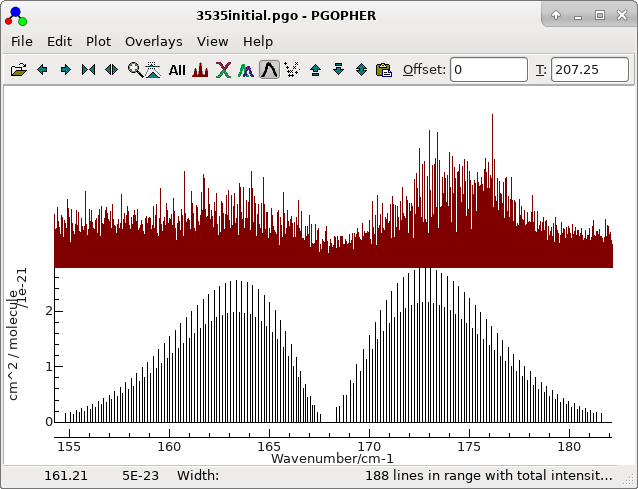
The obvious starting point is with the most abundant species. An
initial simulation is provided in 3535initial.pgo. This
is a standard asymmetric top simulation set up as follows:
The nearest lines window is invaluable in this case. Set it up as
follows.
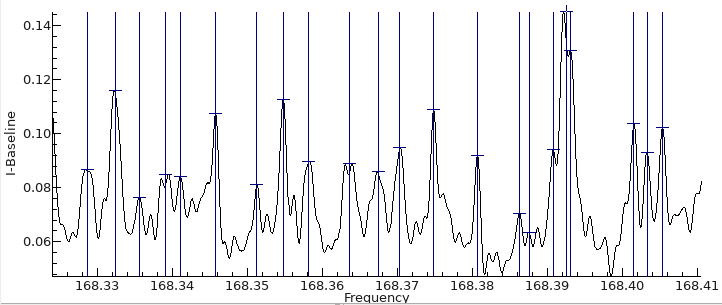
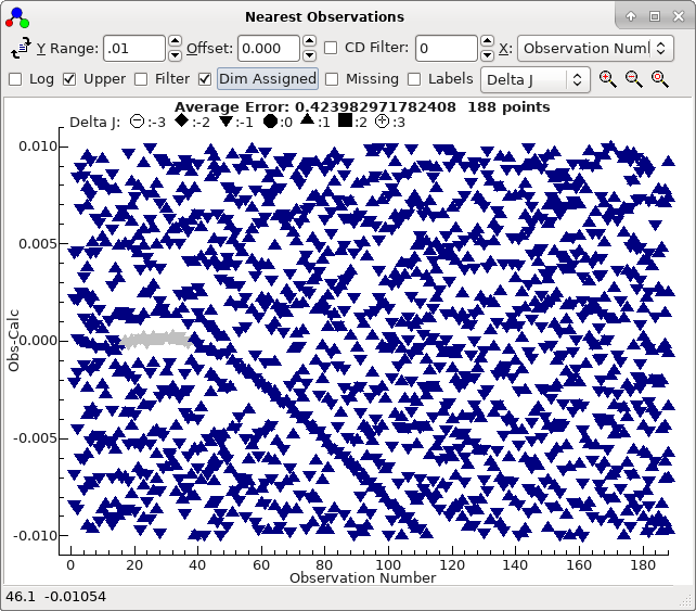
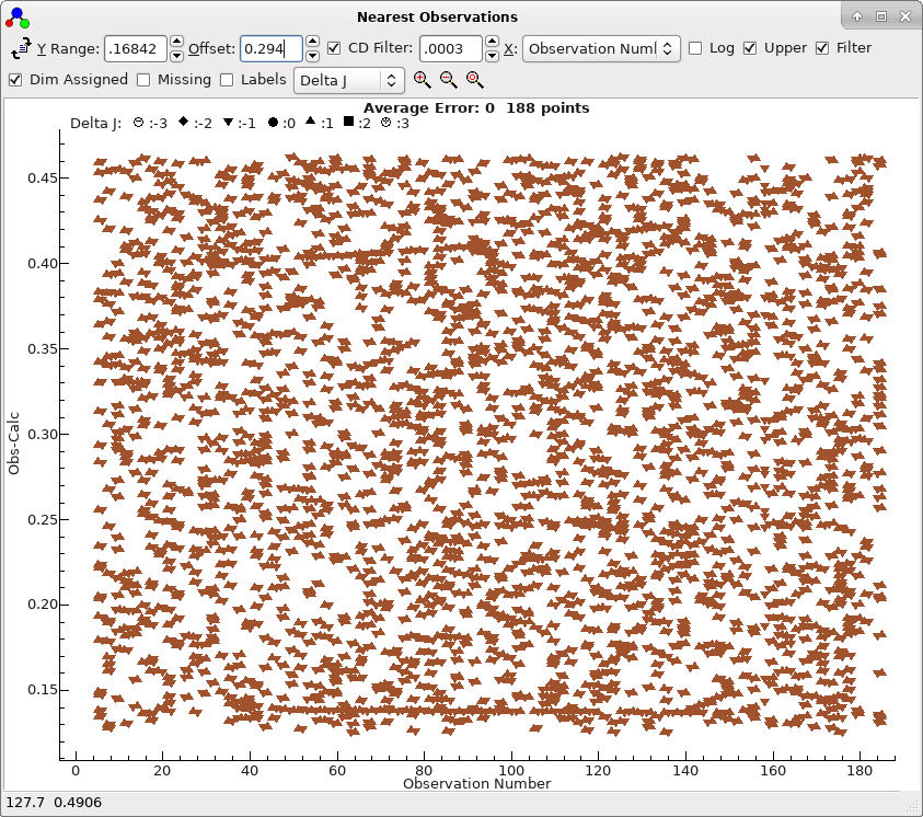
At its simplest this window plots, for each
line in the line list window, a point for each observed line
within the given Y range of that line. If the simulation is
perfect, than a clear horizontal line should appear along the
centre zero line, together with a typically random set of points
either side. An approximately correct simulation should show as
curved lines in the spectrum. This plot is also updated when a
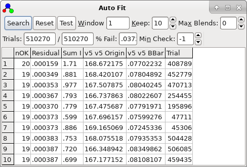
trial is selected by double clicking. In the current case it very
clearly distinguishes between a bad trials (obtained double
clicking on the second row in the autofit window):
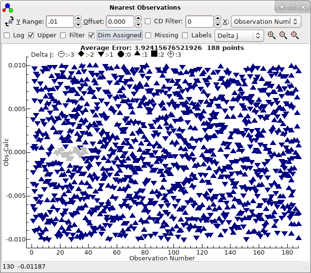
and a good trial (double click on the top row in the trial
window), which shows a clear curve :
To obtain this exact plot "Dim Assigned" has been selected which
plots the assigned points in grey. For this case we have been
lucky, in that the top sorted trial is also the correct one. The
plot indicates that not only are the 21 autofitted transitions
well described by the constants selected, but also many of the
other Ka = 0 transitions lie on a clear trend, if not necessarily
exactly fitted. The file with this fit selected is saved as
3535B.pgo
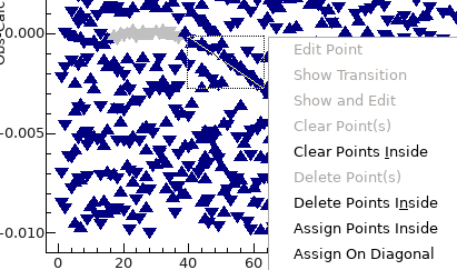
Assignments can be made directly from this window as follows:
- To assign along the curved lines, click and drag with the
mouse so that the diagonal line plotted lies along the line,
right click and select "Assign On Diagonal":
- Repeat as required; if you make a mistake various "Clear
Point..." actions are available by right clicking, and
work in the same way as the residuals window. (The residuals
window will be automatically updated, and it is also possible
to fix problems there.)
- Press "Fit" in the line list window a couple of
times to fit with the new set of assignments. It is clear an
additional parameter is required, and in this case as the
residuals are still curved, so float upper state BDelta.
- This improves the fit, but it is still curved, but so try
floating upper state DJ. This gives an
almost straight line, with an average residual much less that
the line width, so it is probably not worth floating more
parameters at this stage.
The file at this stage is saved as
3535C.pgo.
5. The combination differences filter
An additional check on the assignments is possible from the
nearest lines window, which is to check for combination
differences. This is engaged by checking "CD Filter",
and selecting a non zero value in the box to the right. This
makes use of the known lower state constants (provided "Upper"
is checked) which implies that transition with an upper state in
common have a known separation. The plotting algorithm then work
as follows:
- For each transition in the line list with calculated
position ci,
- For each observed line oj, plot a point
at (ci - oj) if:
- there is a transition in the line list (with position ck)
with the same upper state
- and there is an observed line ol such
that |(ci - oj)-(ck
- ol)| < CD Filter
In the current case the "
CD Filter" value needs to be
quite small to be effective; something in the range of 1/3 of the
line width or less looks good, and eliminates some potential
candidates and confirms others. To limit the assignments to those
confirmed by combination differences:
- Clear all the assignments in the line list window by
clicking on the "Std Dev" column heading to select
the entire column.
- Pressing the delete key to clear all the values.
- Press "Test" to refresh the nearest lines window.
- Reassign the transitions from the nearest lines window as
above.
Refitting fives the file
3535D.pgo.
6. Adding K'a = 1 lines; filtering by state
At this stage we can try adding K'a = 1
lines:
- Use the transitions window as above to add K'a
= 1 lines to the line list window.
- Press "Test" (in the line list window) to update the nearest
lines window.
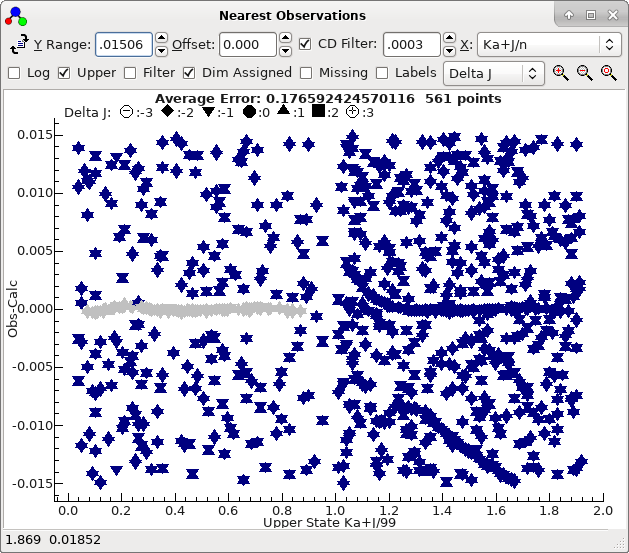
- Separating the lines by both J and Ka
is useful here; try selecting "Ka+J/n" from the X
drop down in the nearest lines window. The x value
plotted is K'a+J'/99 in this case;
the divisor is chosen to be the maximum J' plotted.
- The nearest lines window suggests at first glance that the
K'a lines are in the approximately the right place, but
zooming out a little indicates two sets of lines:
These in fact correspond to two different symmetries. You can
confirm this by changing the "Labels" drop down to "Symmetry"
or, to give a clearer plot:
- Select "Filter" in the nearest lines window. If the
transitions window is showing, then any selection set up will
be applied to the nearest lines window. Here, we want to
select by symmetry, and setting the upper state symmetry to O+
or O- will show one or other of the two curves above. This
avoids assigning to the wrong class of lines, and is used
extensively below.
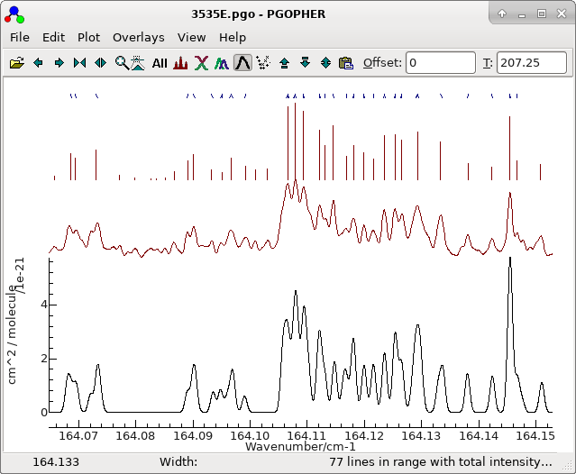
- Both sets of Ka' = 1 lines
can be assigned from the nearest lines window, and A
determined from the upper state by fitting.
- DJK must also be floated to give a
good fit. The file at this stage is saved as 3535E.pgo.
7. Completing the fit
Adding
Ka' = 2 lines to the line list window as
above indicates that these are also in approximately the right
place. To speed things up it is worth adding all the lines to the
line list window, and use filtering for selection. Try:
- In the transitions window, remove all selections, apart from
the selection on strength and ΔJ.
- Press "Add" to add to add all the lines to the line list.
(This adds about 14,000 lines.)
- Scrolling through the Ka' values
indicates an offset steadily increasing with Ka'.
Ka' = 10 looks clear, so try
assigning those transitions.
- Add DK, deltaK and deltaJ
to the fit, and refine the Ka' = 10
assignments.
- Repeat with, say, Ka' = 20, which
is now showing a small error.
- Similarly, repeat with Ka' = 30.
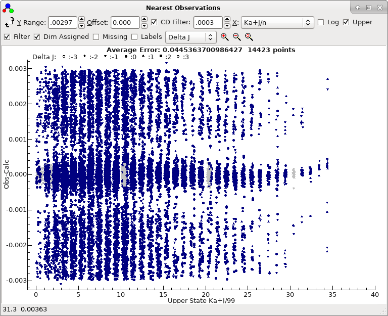
- At this stage almost all the lines are in the right place,
as shown by the nearest lines window if all filtering is
removed:
To obtain this plot the mark size has been reduced by right
clicking on the plot, selecting "Mark Size..." and
entering 50.
- This shows a mild systematic trend. All the lines near the
centre can now be assigned. (Draw a box with the mouse, right
click and select "Assign Points Inside". Note that if
this corresponds to more than one assignment, the assignment
closest to the centre of the box is taken.)
- Allowing the sextic centrifugal distortion constants to
float removes the remaining systematic error, though phiJK
does not seem to be determined.
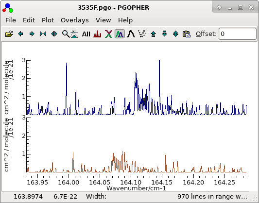
- The simulated spectrum will now show some regions of good
agreement, particularly if one of the sub-band heads is
chosen:
The other structure is examined below.
The file is saved as
3535F.pgo.The
fit yields:
SVD fit: 8937 Observations,  16 Parameters (scaled)
Initial Average Error: 0.00015671996892265
Predicted New Error:   0.00015671996876619
Parameters:
  # Old                 New                 Std Dev   Change/Std Sens    Summary              Name
  1 168.6726199347147   168.6726199356630   6.5669e-6    0.0001  9.79e-7 168.6726199(66)      v5 v5 Origin
  2 .3863882670187941   .3863882670284609   6.7265e-8    0.0001  3.11e-9 0.386388267(67)      v5 v5 A
  3 .07699632041933983  .07699632041453160  9.6864e-9   -0.0005  4.5e-10 0.0769963204(97)     v5 v5 BBar
  4 .01539541616148179  .01539541611604062  2.7760e-8   -0.0016  2.04e-9 0.015395416(28)      v5 v5 BDelta
  5 1.41648688475879e-6 1.41648685071010e-6 1.503e-10   -0.0002  4.7e-12 1.41649(15)e-6       v5 v5 DK
  6 -3.6503095283262e-7 -3.6503087978723e-7 4.834e-11    0.0015  1.6e-12 -3.65031(48)e-7      v5 v5 DJK
  7 4.66951341054434e-8 4.66951203872055e-8 4.906e-12   -0.0028  9.9e-14 4.66951(49)e-8       v5 v5 DJ
  8 1.01758348183677e-7 1.01757477339539e-7 2.132e-10   -0.0041  9.3e-12 1.0176(21)e-7        v5 v5 deltaK
  9 1.15898493061178e-8 1.15898422607635e-8 3.259e-12   -0.0022  9.1e-14 1.15898(33)e-8       v5 v5 deltaJ
 10 2.4676894426514e-11 2.4676709534607e-11 1.336e-13   -0.0014  5.8e-15 2.468(13)e-11        v5 v5 HK
 11 -8.506523576180e-12 -8.506258452295e-12 1.404e-13    0.0019  2.7e-15 -8.51(14)e-12        v5 v5 HKJ
 12 6.0851978998364e-13 6.0845390262616e-13 3.874e-14   -0.0017  5.5e-16 6.08(39)e-13         v5 v5 HJK
 13 3.2546543105758e-14 3.2544072150759e-14 7.059e-16   -0.0035  1.7e-17 3.254(71)e-14        v5 v5 HJ
 14 9.3287154157998e-12 9.3265923563956e-12 1.093e-12   -0.0019  2.4e-14 9.3(11)e-12          v5 v5 phiK
 15 9.1433719046933e-15 8.9794294026524e-15 3.885e-14   -0.0042  1.7e-15 9(39)e-15            v5 v5 phiJK
 16 1.6315297574380e-14 1.6314230317462e-14 3.931e-16   -0.0027  1.4e-17 1.631(39)e-14        v5 v5 phiJ

Correlation Matrix
Largest off-diagonal element = 0.980 at 14,12 = v5 v5 phiK, v5 v5 HJK
       1       2       3       4       5       6       7       8       9      10      11      12      13      14      15      16
  1   1.000
  2  -0.651   1.000
  3  -0.737   0.241   1.000
  4  -0.102  -0.101   0.329   1.000
  5  -0.338   0.803  -0.062  -0.149   1.000
  6  -0.478   0.626   0.370  -0.060   0.136   1.000
  7  -0.423   0.030   0.754   0.495  -0.043  -0.116   1.000
  8  -0.027  -0.028   0.096   0.355   0.060  -0.357   0.653   1.000
  9  -0.113  -0.108   0.364   0.944  -0.101  -0.182   0.629   0.459   1.000
 10  -0.155   0.392  -0.037  -0.029   0.650  -0.178   0.139   0.258   0.055   1.000
 11  -0.093   0.221   0.000  -0.112   0.109   0.363  -0.248  -0.353  -0.182  -0.664   1.000
 12  -0.096   0.059   0.143   0.112   0.015   0.003   0.258   0.310   0.146   0.679  -0.918   1.000
 13  -0.248  -0.037   0.525   0.498   0.001  -0.302   0.935   0.778   0.666   0.267  -0.393   0.353   1.000
 14  -0.019  -0.015   0.052   0.105   0.036  -0.165   0.247   0.368   0.157   0.713  -0.952   0.980   0.387   1.000
 15  -0.033  -0.035   0.115   0.388   0.053  -0.358   0.661   0.970   0.512   0.314  -0.430   0.384   0.827   0.442   1.000
 16  -0.110  -0.105   0.353   0.819  -0.048  -0.281   0.698   0.557   0.946   0.237  -0.387   0.337   0.800   0.369   0.640   1.000
C. C2H235Cl37Cl
The next most abundant species can now be assigned. An initial
simulation is provided in
3537initial.pgo. This
is set up in much the same way as above, with the exception of the
band origin, which is set 2 cm
-1 below the origin
determined above. For this molecule the
PseudoC2v
flag is set, as this speeds up the calculation and also avoids
problems with state assignments at high
J. The analysis
then proceeds as above, with some minor differences. Using exactly
the same autofit selection as above does produce a successful
trial, but at the bottom of the list. (It is trial number 10 if
MinCheck
is set to 0.) There are a couple of approaches that can be taken
to improving fits. Simply changing the two transitions chosen as
trial fit transitions makes a big difference:
- If the trial fit transitions are exchanged between the P
and R transitions (to pP1,11(11) and
pR1,19(19)) at each end of the range,
then the correct trial is not found.
- If the trial fit transitions are moved in one J at
each end (to pR1,11(11) and pR1,18(18))
then the top fit with nOK = 20 is the correct fit.
There is no simple way to predict what is going to work, but it is
straightforward to try a few different fit choices. Alternatively,
a range can be specified for one or more of the parameters. Not
only is this more selective, but this can also speed up the
search, as trials are discarded more quickly. In the current case,
comparing the difference between ground and excited state
constants in the fit above suggests a range of 0.003 cm
-1
would be sensible for
BBar. To search with this
constraint:
- If you have not done so already, press the Reset button
to discard any current autofit assignments
-
To limit the range of a particular
parameter, set the maximum permitted change (+ or -) as the
"Std Dev" for the parameter in the constants
window. In this case set "Std Dev" for the excited
state BBar to 0.003. Tip: to avoid unexpected
constraints, make sure that the standard deviations of all
floated parameters are blank before autofitting. (Click on
the down arrow in the autofit window and select "Clear
Parameter Ranges" to do this.)
A file set up in this way is saved as
3537A.pgo and immediately after
running the autofit as
3537Aafter.pgo.
For this set up, 28% of the trials are rejected and the correct
trial rises to number 7 with
nOk = 20.
Given this start, the fit can then proceed as above. The file
after assigning Ka' = 1 is available as
3537E.pgo, and the final file
as
3537F.pgo. Again the
regions around some band heads show a reasonable match, though not
as good as above as this is a less abundant species.
D. C2H235Cl2 hot
band
The next most prominent band is likely to be the hot band of the
35Cl
2
species, i.e.
v5=2 ←
v5=1,
given the low frequency of the ν5 mode (169 cm
-1)
and the low abundance of the
37Cl
2 species.
To test this, add a hot band to the
35Cl
2
simulation as follows:
- Duplicate the v5 manifold (Right click on the upper v5
in the constants window, select "Copy With Linked Items"
then right click again and select "Paste". In the
rename dialog that is offered, change "v5" to "Copy
of v5" and "Ground" to "v5" to give
the desired transition moment. To avoid confusion, rename both
items in the new manifold to v5=2.)
- For the rotational constants, we use a simple linear
extrapolation involving v5=0 and v5=1.
For the v5=2 origin we use twice the v5=1
value.
- To include transitions with v5 = 1 as the
lower state, Initial for the v5=1
manifold must be set to true.
- This is enough for an initial simulation. To allow the bands
to be distinguished set colours on the states, perhaps navy
on v5=0 and brown for v5=1. Any colour set
elsewhere should be cleared; note that, as described in Determining Colours and J
ranges, the lower state colour takes preference. The
simulation now confirms the hot bad should indeed have
significant intensity:
To prepare the file to fit the hot band:
- Clear all the lines in the linelist
- Fix all parameters, and clear all the standard deviations.
The file at this stage starting from
3535F.pgo is saved as
3535HotInitial.pgo.
We can now proceed as above, starting with the
Ka'=0
lines in the hot band. The only difference is in the transitions
window, in that you will have to use one of the State/Manifold
drop downs to select the hot band. Interestingly, scanning the
offset in the nearset lines window indicates two promising
assignments without further adjustment:
You can use the "Y Range" and "Offset" settings to zoom in on
these individually; note that the mouse wheel can be used to
adjust these. The file at this stage is saved as
3535HotA.pgo.
More detailed investigation of the lower one indicates that it is
actually the cold band, and if you assign from this you will
generate the same assignments derived above for the cold band,
albeit with
J shifted by one. (An additional diagnostic is
that trying to fit from this does not give transitions below
J'
= 20.) The upper one is more promising, and just floating the v5=2
origin and
BBar gives a good fit for
J' = 10-85.
(Tip: the offset on the nearest lines window will need resetting
to zero after the first fit.) The file at this stage is saved as
3535HotB.pgo.
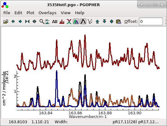
The process given above then works straightforwardly to generate a
final fit with similar quality to the cold bands in
3535HotF.pgo, with promising
simulations in regions where both bands are prominent:
For this plot the lines have been made thicker to bring out the
colours with "
Plot", "
Plot Options", "
Line
Width..." and selecting 2.
E. Other bands
The hot band for C2H235Cl37Cl
can be assigned following the procedures above; the initial file
is available as 3537HotInitial.pgo
and the final file as 3537HotF.pgo.
At this stage some other bands can be considered. The C2H237Cl2
species is probably too weak to see, and an attempt with
estimated constants did not suggest any possible assignments, at
least using the nearest lines plot. This is not surprising,
given that the abundance is 10% of the most abundant
isotopologue. Interestingly, setting up estimated constants for
the v5=3 ← v5=2
(very) hot band for the C2H235Cl2
species gives a shows a possible assignment in the nearest lines
plot for both Ka' = 0 and 1 without a search,
and a reasonable fit for this can be obtained. The initial file
is available as 3535_3-2initial.pgo,
the file with Ka' = 0 and 1assigned as 3535_3-2A.pgo and the
final fit as 3535_3-2F.pgo.
The corresponding C2H235Cl37Cl
band does not seem to be visible.
The appearance of the v5=3 ← v5=2
band, but not the cold C2H237Cl2
species is perhaps surprising, given that both should have
similar intensity at this temperature, and some independent
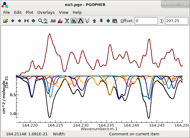
confirmation would be in order. A simulation containing all the
assigned bands makes sense at this point; this can be achieved
by loading one of the files and using "File", "Merge
File...". The result after a little tidying up is in nu5.pgo. With a little hunting,
a few lines can be found that are entirely from the v5=3
← v5=2 band, though most of the assigned
lines are blends. For example see the orange lines in the centre
of the plot. (The black line is the overall simulation.)
For completeness, a file with estimated constants for the C2H237Cl2
cold band and the v5=3 ← v5=2
band for C2H235Cl37Cl
is available as nu5tests.pgo.
References.
- L. A. Leal, J. L. Alonso and A. G. Lesarri, J. Molec.
Spectrosc., 165 368-376 (1994).
 Procedures Automatic Fitting