Worked Example - Refining an ab initio force field for H2O
Importing the ab initio file and setting up the geometry
The first step is to import the ab initio output file. The Molpro output file used here is H2OCAS.out.
- Click on File, Import, l
Matrix... and select the ab initio output file H2OCAS.out.
- Select View, Constants.
You will note that two states have been generated (S0 and S1), corresponding to
the HF and CASSCF stages of the calculation respectively. Only
one of these is required; to use the CASSCF calculation right
click on the first S0
and select "Delete".
Click on "Yes to all" when prompted. To avoid "No
Initial States Set" messages later, make sure that Initial
is set to True in the manifold object (here the upper
S1).
- For clarity, rename some of the items to more meaningful
names. Right click on the item and select "Rename" to do this. The
manifold and state, currently "S1" should both be something like "X", the top "LmatrixImport" item
should be "Water"
and the other "LmatrixImport"
item "H2O".
- Right click on the second "X" and select "Add New
..., z Matrix". This creates a z
matrix object, that allows the more flexible handling of
the geometry.
- Right click on "z Matrix" and select "View ..."
to bring up the z Matrix window.
- Click on "Operate" and select "Load from State"
to set up the z matrix from the coordinates read in from
the ab initio program. For the data file given you will
need to click on "yz" to give the best plot of the
molecule.
Setting up the internal coordinates
The next step is to set up the internal valence coordinates using
an Internal Coordinates object.
Much of this is the same as in Setting
up a simple force field analysis for H2O, except for the
force constants.
- To create the object, right click on the second "X"
and select "Add New ..., Internal Coords".
- Right click on "Internal Coords" and select "View
..." to bring up the Internal
Coordinates Window.
- We now need to enter three Valence
Coordinates; for each we need to enter a type of motion,
and specify 2-4 atoms involved in the motion in the top left
grid.
- The order is not critical, so lets start with an O-H stretch:
- In the first row, click on the first column (under "Mode")
and select "Stretch" from the drop down box.
- Two atoms must be specified in the next two columns - enter
"O" under "Atom k" and "H1" under "Atom
l".
- Click on "Operate" and select "Check" to
check and update the plot if necessary. (Moving to a different
row using the arrow keys also triggers a this process.) Note
that error messages will appear in the plot title; you may
have noticed, for example, "1:3:Missing Atom 2"
appear after you entered "O", which indicates an error
(missing atom) associated with row 1 column 3. If the mode is
set up correctly, the plot should show the stretch when the
cursor is on the top row.
- Enter the second OH stretch in the next row of both grids: in
the left grid add "Stretch", "O" and "H2"
- The final mode is the bend in the next row, for which 3 atoms
must be specified: in the left grid add "Bend", "H1",
"O" and "H2". Note that the second atom ("Atom
l") is the central atom.
Setting up the force constants
The next step is to calculate the force constants in valence
coordinates from the l matrix and frequencies read in.
- Click on "Operate" and select "Calculate f matrix
from l" to print the force constant matrix in the log
window with some details of the calculation from the l
matrix and frequencies.
- If the force constant matrix is OK, click on "Operate"
and select "Set f matrix from l" to populate
the grid in the top right with the force constants.
- The calculation may generate several very small values that
you may want to set to zero. The easiest way of doing this is
click on "Operate" and select "Sort f
matrix by Value". This puts the smallest values at the
bottom of the grid, where they can be deleted as a group. (For
the sample file given here all the values look significant). To
revert to the original sort order click on "Operate"
and select "Sort f matrix by Mode".
- For refining the force field, it is convenient to express the
force constants as variables. There are various ways to do this;
here we start by using the same variables as in Setting up a simple force field
analysis for H2O. To set the variables up, right click on
"Internal Coords" and select "Add Parameter...".
Enter kstretch kbend kstrstr kstrbend
when prompted. (The names are arbitrary - use whatever names are
most convenient.)
- The variables will now be visible in the constants window, set
to the default values of zero. Copy and paste the values from
the top right grid in internal coordinates window - kstretch
will be the 11 and 2 2 value, for example.
- The numerical values in the top right window should then be
replaced by the variable. The simplest approach would be to
replace the value with the variable, so replace the 1 1
and 2 2 values by kstretch. However, to
allow for a uniform scaling of the force constants we input it
as ks*kstretch. The will create a variable, ks,
that should be initialized to 1. After setting the cell, click
on "Operate" and "Check" to force the generation of the
variable. This will create the ks variable; set the
value to 1.
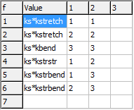
- Repeat the process for the other force constants.
The result should be a force constant matrix that looks like this:

The file is available as
H2Oabf1.pgo. If required a
similar process can be followed for the
z matrix, but this
requires a little more work as the atom positions are imported in
Cartesian coordinates. Conversion to the more convenient bond
length/bond angle format must be done manually. For the
current case the z Matrix given in used in the related worked
example
Setting up a simple force
field analysis for H2O can be used, and the necessary bond
length and bond angle can be picked out of the
ab intio
output.
Refining the force field
We can now fit the force constants to the
observed vibrational frequencies, for which we use the values of
ν1 = 3656.65, ν2 = 1594.59, and ν3
= 3755.79 given in Table XI of "Rotation-Vibration Spectra of
Deuterated Water Vapor", W. S. Benedict, N. Gailar, and Earle K.
Plyler, J. Chem. Phys. 24, 1139 (1956) http://dx.doi.org/10.1063/1.1742731.
The first step is assigning the vibrational modes; the
observations are sorted by symmetry, symmetric modes first, and
then frequency but the calculated modes are only sorted by
frequency. The current calculation does not make any use of
symmetry, so a manual step is required to assign the observed and
calculated frequencies. The calculated normal modes are best
visualised in the l Matrix Window;
right click on the lower "X" and select "l matrix..."
to bring it up. Click on "yz" to select the best plot for
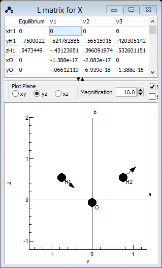
showing vibrations. Clicking in a particular column in the top
grid plots the selected mode; clicking on the "v1" column
for example gives the following:

which clearly shows that v1 is the
asymmetric stretch, ν3 in the experimental paper.
Similarly v2 is the symmetric stretch, ν1in
the experimental paper and v3 is the bend. This
information can be presented to PGOPHER by adding the following
lines to an observation file:
Parameter X.v1.Omega = 3755.79
Parameter X.v2.Omega = 3656.65
Parameter X.v3.Omega = 1594.59
This is available in H2Oab1.obs. To use this file:
- Open the log window ("View,
Log...") if it is not open already.
- The text box at the top needs to contain the file name; drag
and drop the file onto the window, or use the browse button to
the right of the text box to bring up a file browsing dialog.
- Make sure the fit type at the top left is set to "Line".
- At this stage no parameters have been floated, so pressing the
"Fit" button will simply print out a set of observed
and calculated values, that can be used to check that the file
has been set up correctly. In this case we have:
Residuals before fit
    J'S' #'    J"S" #"     Observed    Calculated      Obs-Calc StdDev
v1.Omega                  3755.7900     3833.4000      -77.6100 1        :   4:H2Oab1.obs
v2.Omega                  3656.6500     3721.3600      -64.7100 1        :   5:H2Oab1.obs
v3.Omega                  1594.5900     1715.2800     -120.6900 1        :   6:H2Oab1.obs

3 Observations,  0 Parameters
Average Error: 90.8786230550515
indicating that the vibrations are assigned correctly.
- The obvious parameter to float is the scaling variable ks.
To allow this to float, click on "Internal Coords" in
the constants window and change the "no" by ks
to "yes" by clicking on the "no".
- Pressing the "Fit" button will now carry out one
cycle of least squares fitting. The initial observed and
calculated values are printed out, followed by an estimate of
better values for the floated parameters. As this is a
non-linear fit several cycles will be required for convergence -
keep pressing the fit button until the values converge. In this
case only 1 or 2 cycles are required for convergence. (If the
values diverge use the undo fit button to step back through the
fit cycles, and float less parameters or make some manual
changes to the floated parameters.) The final fit cycle gives a
reasonable fit:. In this case we have:
Residuals before fit
    J'S' #'    J"S" #"     Observed    Calculated      Obs-Calc StdDev
v1.Omega                  3755.7900     3742.6547       13.1353 1        :   4:H2Oab1.obs
v2.Omega                  3656.6500     3633.2669       23.3831 1        :   5:H2Oab1.obs
v3.Omega                  1594.5900     1674.6754      -80.0854 1        :   6:H2Oab1.obs

3 Observations,  1 Parameters
Initial Average Error: 59.7200825208321
Predicted New Error:   59.720082520669
Parameters:
  # Old                 New                 Std Dev   Change/Std Sens    Summary              Name
  1 .9532157999599624   .9532158686557101   .02078263    0.0000  .0036   0.953(21)            Internal Coords ks
- The fit could be improved in various ways; the obvious one is
to float the kbend force constant as well. More
experimental information, from other isotopes for example, could
also be added; see Setting up a
combined force field analysis for H2O and D2O for how to
do this.

